better-satcen-00001 data pipeline results (Sentinel-2 Vegetation and Water themtic index) : loading from pickle file and exploiting
This Notebook shows how to: * reload better-satcen-00001 data pipeline results previously stored in a pickle file * Create a new dataframe with data values cropped over the area of interest * Plot an RGB * Create a geotif
Import needed modules
In [1]:
import pandas as pd
from geopandas import GeoDataFrame
import gdal
import numpy as np
from shapely.geometry import Point
from shapely.geometry import Polygon
import matplotlib
import matplotlib.pyplot as plt
from PIL import Image
%matplotlib inline
from shapely.wkt import loads
from shapely.geometry import box
from urlparse import urlparse
import requests
Read picke data file
In [2]:
pickle_filename = 'better-satcen-00001_May_2018_Albania-GreeceBorder.pkl'
In [3]:
results = GeoDataFrame(pd.read_pickle(pickle_filename))
In [4]:
results.head()
Out[4]:
| enclosure | enddate | identifier | self | startdate | title | wkt | |
|---|---|---|---|---|---|---|---|
| 0 | https://store.terradue.com/better-satcen-00001... | 2018-05-22 09:30:29.027 | 0712a0fdc17bad31138dfef3f6d57a6cb66962ea | https://catalog.terradue.com//better-satcen-00... | 2018-05-22 09:30:29.027 | S2B_MSIL2A_20180522T093029_N0207_R136_T34TEK_2... | POLYGON((20.9997634361085 39.661229210097,21.2... |
| 1 | https://store.terradue.com/better-satcen-00001... | 2018-05-22 09:30:29.027 | 07fb7271ad6b5c5d2b23ff305c617c0a532926bc | https://catalog.terradue.com//better-satcen-00... | 2018-05-22 09:30:29.027 | S2B_MSIL2A_20180522T093029_N0207_R136_T34TEK_2... | POLYGON((20.9997634361085 39.661229210097,21.2... |
| 2 | https://store.terradue.com/better-satcen-00001... | 2018-05-22 09:30:29.027 | 15412a409b5f269b90a6c4edd71a70355830ed6f | https://catalog.terradue.com//better-satcen-00... | 2018-05-22 09:30:29.027 | S2B_MSIL2A_20180522T093029_N0207_R136_T34TDL_2... | POLYGON((19.8899808364281 40.5626923867771,21.... |
| 3 | https://store.terradue.com/better-satcen-00001... | 2018-05-22 09:30:29.027 | 238107f531ed150ebb3ee0763d3d690ec791b305 | https://catalog.terradue.com//better-satcen-00... | 2018-05-22 09:30:29.027 | S2B_MSIL2A_20180522T093029_N0207_R136_T34TEK_2... | POLYGON((20.9997634361085 39.661229210097,21.2... |
| 4 | https://store.terradue.com/better-satcen-00001... | 2018-05-22 09:30:29.027 | 2eebf44a805a2de437e839a6245260e6c2449948 | https://catalog.terradue.com//better-satcen-00... | 2018-05-22 09:30:29.027 | S2B_MSIL2A_20180522T093029_N0207_R136_T34TEK_2... | POLYGON((20.9997634361085 39.661229210097,21.2... |
Credentials for ellip platform access
- Provide here your ellip username and api key for platform access
In [5]:
import getpass

user = getpass.getpass("Enter your username:")
In [6]:
api_key = getpass.getpass("Enter the API key:")
Define filter parameters
Time of interest
In [7]:
mydates = ['2018-05-22 09:30:29.027','2018-05-14 09:20:31.024000', '2018-05-12 09:30:29.027000000', '2018-05-09 09:20:29.027000', '2018-05-07 09:30:41.024000', '2018-05-02 09:30:39.027000']
Area of interest
- The user can choose to define an AOI selecting a Point and a buffer size used to build a squared polygon around that point
In [8]:
point_of_interest = Point(20.951, 40.768)
In [9]:
buffer_size = 0.07
In [10]:
aoi_wkt1 = box(*point_of_interest.buffer(buffer_size).bounds)
In [11]:
aoi_wkt1.wkt
Out[11]:
'POLYGON ((21.021 40.698, 21.021 40.838, 20.881 40.838, 20.881 40.698, 21.021 40.698))'
- Or creating a Polygon from a points list (in this case this is exactly the Albania/Greece border reference AOI)
In [12]:
aoi_wkt2 = Polygon([(21.2961, 39.58638), (21.2961, 41.032), (19.8978, 41.032), (19.8978, 39.58638), (21.2961, 39.58638)])
In [13]:
aoi_wkt2.wkt
Out[13]:
'POLYGON ((21.2961 39.58638, 21.2961 41.032, 19.8978 41.032, 19.8978 39.58638, 21.2961 39.58638))'
Create a new dataframe with data values
- Get the subframe data values related to selected tiles and bands, and create a new GeoDataFrame having the original metadata stack with the specific bands data extended info (data values, size, and geo projection and transformation).
Define auxiliary methods to create new dataframe
- The first method gets tile reference, bands numbers, cropping flag, AOI cropping area and returns the related n bands data array with related geospatial infos
- If crop = False the original bands extent is returned
In [14]:
def get_bands_as_array(url,crop,bbox):

    #[-projwin ulx uly lrx lry]
    ulx, uly, lrx, lry = bbox[0], bbox[3], bbox[2], bbox[1]

    output = '/vsimem/clip.tif'

    ds = gdal.Open('/vsicurl/%s' % url)
    ds = gdal.Translate(output, ds, projWin = [ulx, uly, lrx, lry], projWinSRS = 'EPSG:4326')
    ds = None

    ds = gdal.Open('/vsimem/clip.tif')
    band = ds.GetRasterBand(1)

    w = band.XSize
    h = band.YSize
    geo_transform = ds.GetGeoTransform()
    projection = ds.GetProjection()

    data = band.ReadAsArray(0, 0, w, h).astype(np.float)

    data[data==-9999] = np.nan

    ds = None
    band = None

    return data,geo_transform,projection,w,h
- The second one selects the data to be managed (only the actual result related to the selected tile) and returns a new GeoDataFrame containing the requested bands extended info with the original metadata set
In [15]:
def get_info(row, user, api_key, crop=False, bbox=None):

    print 'Getting band %s' %(row['title'])

    band_name = row['title'].rsplit('CROP_', 1)[1].split('.')[0]

    parsed_url = urlparse(row['enclosure'])

    url = '%s://%s:%s@%s/api%s' % (list(parsed_url)[0], user, api_key, list(parsed_url)[1], list(parsed_url)[2])

    bands,geo_transform,projection,w,h = get_bands_as_array(url,crop,bbox)

    extended_info = dict()

    extended_info['band'] = band_name
    extended_info['data'] = bands
    extended_info['geo_transform'] = geo_transform
    extended_info['projection'] = projection
    extended_info['xsize'] = w
    extended_info['ysize'] = h

    series = pd.Series(extended_info)
    print 'Get data values for %s : DONE' %row['title']
    return series
- Define the reference tiles
In [16]:
ref_tiles = ['T34TDK', 'T34TEK', 'T34TDL']
- Define the selected bands (among the available ones) to be exploited
In [17]:
available_bands = ['ndwi', 'ndvi', 'quality_cloud_confidence', 'quality_snow_confidence', 'quality_scene_classification', 'B2', 'B3', 'B4', 'B5', 'B6', 'B7', 'B8', 'B8A', 'B11', 'B12']

selected_bands = ['ndwi', 'ndvi','B2','B3','B4']
- Select from metadataframe a subframe related to
- a single datetime
- multiple georeferenced tiles of interest
- selected bands
In [18]:
selected_bands = ['ndwi', 'ndvi','B2','B3','B4']

mydate_results = results[(results['startdate'] == mydates[0]) &
                         (results.apply(lambda row: row['title'].rsplit('CROP_', 1)[1].split('.')[0] in selected_bands, axis=1)) &
                         (results.apply(lambda row: ref_tiles[2] in row['title'], axis=1))]

mydate_results = mydate_results.merge(mydate_results.apply(lambda row: get_info(row, user, api_key, True, list(aoi_wkt1.bounds)), axis=1), left_index=True, right_index=True)
Getting band S2B_MSIL2A_20180522T093029_N0207_R136_T34TDL_20180522T121543_PA_CROP_ndwi.tif
Get data values for S2B_MSIL2A_20180522T093029_N0207_R136_T34TDL_20180522T121543_PA_CROP_ndwi.tif : DONE
Getting band S2B_MSIL2A_20180522T093029_N0207_R136_T34TDL_20180522T121543_PA_CROP_ndvi.tif
Get data values for S2B_MSIL2A_20180522T093029_N0207_R136_T34TDL_20180522T121543_PA_CROP_ndvi.tif : DONE
Getting band S2B_MSIL2A_20180522T093029_N0207_R136_T34TDL_20180522T121543_PA_CROP_B4.tif
Get data values for S2B_MSIL2A_20180522T093029_N0207_R136_T34TDL_20180522T121543_PA_CROP_B4.tif : DONE
Getting band S2B_MSIL2A_20180522T093029_N0207_R136_T34TDL_20180522T121543_PA_CROP_B2.tif
Get data values for S2B_MSIL2A_20180522T093029_N0207_R136_T34TDL_20180522T121543_PA_CROP_B2.tif : DONE
Getting band S2B_MSIL2A_20180522T093029_N0207_R136_T34TDL_20180522T121543_PA_CROP_B3.tif
Get data values for S2B_MSIL2A_20180522T093029_N0207_R136_T34TDL_20180522T121543_PA_CROP_B3.tif : DONE
In [19]:
mydate_results.head()
Out[19]:
| enclosure | enddate | identifier | self | startdate | title | wkt | band | data | geo_transform | projection | xsize | ysize | |
|---|---|---|---|---|---|---|---|---|---|---|---|---|---|
| 6 | https://store.terradue.com/better-satcen-00001... | 2018-05-22 09:30:29.027 | 568c349b9dc75551e4ce5bfcd78331bbe836b3e5 | https://catalog.terradue.com//better-satcen-00... | 2018-05-22 09:30:29.027 | S2B_MSIL2A_20180522T093029_N0207_R136_T34TDL_2... | POLYGON((19.8899808364281 40.5626923867771,21.... | ndwi | [[10850.0, 10492.0, 10808.0, 10545.0, 11087.0,... | (489960.0, 10.0, 0.0, 4520790.0, 0.0, -10.0) | PROJCS["WGS 84 / UTM zone 34N",GEOGCS["WGS 84"... | 1181 | 1555 |
| 18 | https://store.terradue.com/better-satcen-00001... | 2018-05-22 09:30:29.027 | f98960e9502a48c0e828c09286607409e34b910b | https://catalog.terradue.com//better-satcen-00... | 2018-05-22 09:30:29.027 | S2B_MSIL2A_20180522T093029_N0207_R136_T34TDL_2... | POLYGON((19.8899808364281 40.5626923867771,21.... | ndvi | [[11299.0, 11599.0, 12047.0, 12331.0, 12509.0,... | (489960.0, 10.0, 0.0, 4520790.0, 0.0, -10.0) | PROJCS["WGS 84 / UTM zone 34N",GEOGCS["WGS 84"... | 1181 | 1555 |
| 26 | https://store.terradue.com/better-satcen-00001... | 2018-05-22 09:30:29.027 | 5a40bae355f9fea6c4122adf6e0e97a202235689 | https://catalog.terradue.com//better-satcen-00... | 2018-05-22 09:30:29.027 | S2B_MSIL2A_20180522T093029_N0207_R136_T34TDL_2... | POLYGON((19.8899808364281 40.5626923867771,21.... | B4 | [[4188.0, 3665.0, 3079.0, 2751.0, 2661.0, 2773... | (489960.0, 10.0, 0.0, 4520790.0, 0.0, -10.0) | PROJCS["WGS 84 / UTM zone 34N",GEOGCS["WGS 84"... | 1181 | 1555 |
| 27 | https://store.terradue.com/better-satcen-00001... | 2018-05-22 09:30:29.027 | 661b503be3240860f0a99975f61a70ad255597b9 | https://catalog.terradue.com//better-satcen-00... | 2018-05-22 09:30:29.027 | S2B_MSIL2A_20180522T093029_N0207_R136_T34TDL_2... | POLYGON((19.8899808364281 40.5626923867771,21.... | B2 | [[4241.0, 3696.0, 3080.0, 2722.0, 2758.0, 2684... | (489960.0, 10.0, 0.0, 4520790.0, 0.0, -10.0) | PROJCS["WGS 84 / UTM zone 34N",GEOGCS["WGS 84"... | 1181 | 1555 |
| 31 | https://store.terradue.com/better-satcen-00001... | 2018-05-22 09:30:29.027 | 7f6a9e0fac87968d4d090d1279a7f008b1ee88a1 | https://catalog.terradue.com//better-satcen-00... | 2018-05-22 09:30:29.027 | S2B_MSIL2A_20180522T093029_N0207_R136_T34TDL_2... | POLYGON((19.8899808364281 40.5626923867771,21.... | B3 | [[4328.0, 3711.0, 3236.0, 2829.0, 2795.0, 2848... | (489960.0, 10.0, 0.0, 4520790.0, 0.0, -10.0) | PROJCS["WGS 84 / UTM zone 34N",GEOGCS["WGS 84"... | 1181 | 1555 |
*Or*
- Select from metadataframe a subframe related ndvi and ndwi of different tiles in the same date:
- Show data values of NDVI bands
In [20]:
mydate_results[mydate_results['band'] == 'ndvi']['data'].values
Out[20]:
array([ array([[ 11299.,  11599.,  12047., ...,   9400.,   9345.,   9732.],
       [ 11615.,  11920.,  12372., ...,   9732.,   9411.,   9727.],
       [ 11706.,  11853.,  12393., ...,   9686.,   9816.,   9953.],
       ...,
       [ 15029.,  14047.,  15687., ...,  16792.,  17198.,  17284.],
       [ 15227.,  13962.,  16377., ...,  16928.,  17042.,  17412.],
       [ 15799.,  14860.,  16004., ...,  17046.,  16956.,  17106.]])], dtype=object)
Plotting data and exporting geotif
Plot data
Plot all the selected bands
In [21]:
bands = None

bands =  mydate_results['data'].values
titles = mydate_results['title'].values

numbands = len(bands)
print numbands

for i in range(numbands):
    bmin = bands[i].min()
    bmax = bands[i].max()
    if bmin != bmax:
        bands[i] = (bands[i] - bmin)/(bmax - bmin) * 255
    else:
        print 'WARNING bmin %s = bmax %s (%i)!' %(bmin, bmax,i)
5
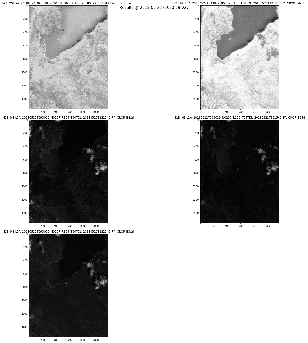
- Plot the selected bands separately
In [22]:
fig = plt.figure(figsize=(20,20))
fig.suptitle('Results @ %s' % (mydates[0]), fontsize=16)

for i in range(numbands):
    a = fig.add_subplot(3, 2, i+1)
    #
    imgplot = plt.imshow(bands[i].astype(np.uint8),
                         cmap='gray')
    a.set_title(titles[i])

plt.tight_layout()
fig = plt.gcf()
plt.show()

fig.clf()
plt.close()
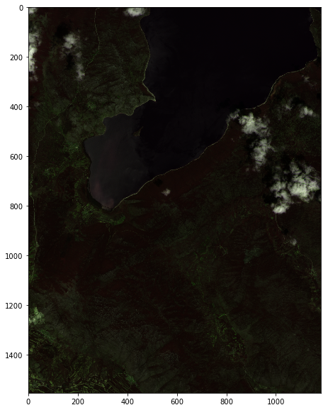
- Plot them as an RGB
In [23]:
rgb_bands = (bands[4],bands[2],bands[3])

rgb_uint8 = np.dstack(rgb_bands).astype(np.uint8)

width = 10
height = 10
plt.figure(figsize=(width, height))
img = Image.fromarray(rgb_uint8)
imgplot = plt.imshow(img)
Export a Geotiff
In [24]:
band_number = 3
cols = mydate_results['xsize'].values[0]
rows = mydate_results['ysize'].values[0]

print (cols,rows)

geo_transform = mydate_results['geo_transform'].values[0]
projection = mydate_results['projection'].values[0]

drv = gdal.GetDriverByName('GTiff')

ds = drv.Create('export.tif', cols, rows, band_number, gdal.GDT_Float32)

ds.SetGeoTransform(geo_transform)
ds.SetProjection(projection)

ds.GetRasterBand(1).WriteArray(bands[0], 0, 0)
ds.GetRasterBand(2).WriteArray(bands[1], 0, 0)
ds.GetRasterBand(3).WriteArray(bands[2], 0, 0)
ds.FlushCache()
(1181, 1555)
Download functionalities
Download a product
- Define the download function
In [25]:
def get_product(url, dest, api_key):

    request_headers = {'X-JFrog-Art-Api': api_key}

    r = requests.get(url, headers=request_headers)

    open(dest, 'wb').write(r.content)

    return r.status_code
- Get the reference download endpoint for the product related to the first date
In [26]:
enclosure = mydate_results[(mydate_results['startdate'] == mydates[0])]['enclosure'].values[0]

enclosure
Out[26]:
'https://store.terradue.com/better-satcen-00001/_results/workflows/ec_better_ewf_satcen_01_01_01_ewf_satcen_01_01_01_0_13/run/95ac10ac-315d-11e9-a8e6-0242ac11000f/0012261-181221095105003-oozie-oozi-W/b1a47f4d-ed2a-46cb-95c2-9d32287eb7dd/S2B_MSIL2A_20180522T093029_N0207_R136_T34TDL_20180522T121543_PA_CROP_ndwi.tif'
In [27]:
output_name = mydate_results[(mydate_results['startdate'] == mydates[0])]['title'].values[0]

output_name
Out[27]:
'S2B_MSIL2A_20180522T093029_N0207_R136_T34TDL_20180522T121543_PA_CROP_ndwi.tif'
In [28]:
get_product(enclosure,
            output_name,
            api_key)
Out[28]:
200
Bulk Download
- Define the bulk download function
In [29]:
def get_product_bulk(row, api_key):

    return get_product(row['enclosure'],
                       row['title'],
                       api_key)
- Download all the products related to a chosen date
In [30]:
date_results = results[(results['startdate'] == mydates[0])]
date_results.apply(lambda row: get_product_bulk(row, api_key), axis=1)
Out[30]:
0      200
1      200
2      200
3      200
4      200
5      200
6      200
7      200
8      200
9      200
10     200
11     200
12     200
13     200
14     200
15     200
16     200
17     200
18     200
19     200
20     200
21     200
22     200
23     200
24     200
25     200
26     200
27     200
28     200
29     200
      ...
75     200
76     200
77     200
78     200
79     200
80     200
81     200
82     200
83     200
84     200
85     200
86     200
87     200
88     200
89     200
90     200
91     200
92     200
93     200
94     200
95     200
96     200
97     200
98     200
99     200
100    200
101    200
102    200
103    200
104    200
Length: 105, dtype: int64