better-wfp-00002 data pipeline results (Sentinel-1 Coherence timeseries): loading from pickle file and exploiting
This Notebook shows how to: * reload better-wfp-00002 data pipeline results previously stored in a pickle file * Create a new dataframe with data values cropped over the area of interest * Plot an RGB * Create a geotif
Import needed modules
In [1]:
import pandas as pd
from geopandas import GeoDataFrame
import gdal
import numpy as np
from shapely.geometry import Point
from shapely.geometry import Polygon
import matplotlib
import matplotlib.pyplot as plt
from PIL import Image
%matplotlib inline
from shapely.wkt import loads
from shapely.geometry import box
from urlparse import urlparse
import requests
Read picke data file
In [2]:
pickle_filename = 'better-wfp-00002_validations.pkl'
In [3]:
results = GeoDataFrame(pd.read_pickle(pickle_filename))
In [4]:
results.head(25)
Out[4]:
| enclosure | enddate | identifier | self | startdate | title | wkt | |
|---|---|---|---|---|---|---|---|
| 0 | https://store.terradue.com/better-wfp-00002/_r... | 2017-01-17 03:50:08 | 585efc39a7c4b1e6df4689c41123be2f17cecd8e | https://catalog.terradue.com//better-wfp-00002... | 2017-01-11 03:49:20 | S1_COH_20170117035008_20170111034920_C2F1_116E... | POLYGON((29.0590832889222 7.90674554216732 |
| 1 | https://store.terradue.com/better-wfp-00002/_r... | 2017-01-17 03:50:08 | 9221e259f96e36c100465124b204dd332d34a64a | https://catalog.terradue.com//better-wfp-00002... | 2017-01-11 03:49:20 | Reproducibility notebook used for generating S... | POLYGON((29.0590832889222 7.90674554216732 |
| 2 | https://store.terradue.com/better-wfp-00002/_r... | 2017-01-17 03:50:08 | 94d07730ae194ef7262a807bf2bc08f293dad340 | https://catalog.terradue.com//better-wfp-00002... | 2017-01-11 03:49:20 | Reproducibility stage-in notebook for Sentinel... | POLYGON((29.0590832889222 7.90674554216732 |
| 3 | https://store.terradue.com/better-wfp-00002/_r... | 2017-01-11 03:49:20 | 7c31ba69c43771b536906eb85226371195e7c1b1 | https://catalog.terradue.com//better-wfp-00002... | 2017-01-05 03:50:00 | Reproducibility stage-in notebook for Sentinel... | POLYGON((29.1590086933083 8.57426607119175 |
| 4 | https://store.terradue.com/better-wfp-00002/_r... | 2017-01-11 03:49:20 | e32e3854009a02076089eb4e2164cfc508cd1c07 | https://catalog.terradue.com//better-wfp-00002... | 2017-01-05 03:50:00 | S1_COH_20170111034920_20170105035000_116E_0110... | POLYGON((29.1590086933083 8.57426607119175 |
| 5 | https://store.terradue.com/better-wfp-00002/_r... | 2017-01-11 03:49:20 | ee7ac38b242d1eb8ec8a3eae619a1ccd62e33096 | https://catalog.terradue.com//better-wfp-00002... | 2017-01-05 03:50:00 | Reproducibility notebook used for generating S... | POLYGON((29.1590086933083 8.57426607119175 |
Credentials for ellip platform access
- Provide here your ellip username and api key for platform access
In [5]:
import getpass

user = getpass.getpass("Enter you ellip username:")
api_key = getpass.getpass("Enter the API key:")
Define filter parameters
Time of interest
In [6]:
mydates = ['2017-01-11 03:49:20', '2017-01-05 03:50:00']
Area of interest (two approaches to determine AOI)
- The user can choose to define an AOI selecting a Point and a buffer size used to build a squared polygon around that point
In [7]:
point_of_interest = Point(28.478, 9.083)
In [8]:
buffer_size = 0.07
In [9]:
aoi_wkt1 = box(*point_of_interest.buffer(buffer_size).bounds)
In [10]:
aoi_wkt1.wkt
Out[10]:
'POLYGON ((28.548 9.013, 28.548 9.153, 28.408 9.153, 28.408 9.013, 28.548 9.013))'
- Or creating a Polygon from a points list (in this case this is a point inside the intersect of all results’ polygons)
In [11]:
aoi_wkt2 = Polygon([(29.0590832889222, 7.90674554216732), (29.0590832889222, 9.73355950395278), (28.0078747434455, 9.73355950395278), (28.0078747434455 ,7.90674554216732), (29.0590832889222 ,7.90674554216732)])
In [12]:
aoi_wkt2.wkt
Out[12]:
'POLYGON ((29.0590832889222 7.90674554216732, 29.0590832889222 9.73355950395278, 28.0078747434455 9.73355950395278, 28.0078747434455 7.90674554216732, 29.0590832889222 7.90674554216732))'
Create a new dataframe with data values
- Get the subframe data values related to selected tiles and the selected band, and create a new GeoDataFrame having the original metadata stack with the specific band data extended info (data values, size, and geo projection and transformation).
Define auxiliary methods to create new dataframe
- The first method gets download reference, band number, cropping flag, AOI cropping area and returns the related band data array with related original geospatial infos
- If crop = False the original band extent is returned
In [13]:
def get_band_as_array(url,crop,bbox):

    output = '/vsimem/clip.tif'

    ds = gdal.Open('/vsigzip//vsicurl/%s' % url)

    if crop == True:
        ulx, uly, lrx, lry = bbox[0], bbox[3], bbox[2], bbox[1]
        ds = gdal.Translate(output, ds, projWin = [ulx, uly, lrx, lry], projWinSRS = 'EPSG:4326')
        print 'data cropping : DONE'
    else:

        ds = gdal.Translate(output, ds)
    ds = None
    ds = gdal.Open(output)
    w = ds.GetRasterBand(1).XSize
    h = ds.GetRasterBand(1).YSize
    geo_transform = ds.GetGeoTransform()
    projection = ds.GetProjection()


    data = ds.GetRasterBand(1).ReadAsArray(0, 0, w, h).astype(np.float)

    data[data==-9999] = np.nan

    ds = None

    return data,geo_transform,projection,w,h
- The second one selects the data to be managed (only the actual results related to the filtered metadata) and returns a new GeoDataFrame containing the requested bands extended info with the original metadata set
In [14]:
def get_GDF_with_datavalues(row, user, api_key,  crop=False, bbox=None):


    parsed_url = urlparse(row['enclosure'])

    url = '%s://%s:%s@%s/api%s' % (list(parsed_url)[0], user, api_key, list(parsed_url)[1], list(parsed_url)[2])

    data,geo_transform,projection,w,h = get_band_as_array(url,crop,bbox)

    extended_info = dict()

    extended_info['data'] = data
    extended_info['band'] = row['title']
    extended_info['geo_transform'] = geo_transform
    extended_info['projection'] = projection
    extended_info['xsize'] = w
    extended_info['ysize'] = h


    print 'Get data values for %s : DONE!' %row['title']
    return extended_info
- Select from metadataframe a subframe containing the geotiff results of the datetimes of interest
In [15]:
mydate_results = results[(results.apply(lambda row: 'TIFF' in row['title'], axis=1)) & (results.apply(lambda row: row['startdate'] in pd.to_datetime(mydates) , axis=1))]
*PARAMETERS*
- crop = True|False
if crop=False the bbox can be omitted
In [16]:
myGDF = GeoDataFrame()
for row in mydate_results.iterrows():
    myGDF = myGDF.append(get_GDF_with_datavalues(row[1], user, api_key, True, bbox=aoi_wkt1.bounds), ignore_index=True)
data cropping : DONE
Get data values for S1_COH_20170117035008_20170111034920_C2F1_116E_9C9D Coherence TIFF generated for Sentinel-1 : DONE!
data cropping : DONE
Get data values for S1_COH_20170111034920_20170105035000_116E_0110 Coherence TIFF generated for Sentinel-1 : DONE!
In [17]:
myGDF
Out[17]:
| band | data | geo_transform | projection | xsize | ysize | |
|---|---|---|---|---|---|---|
| 0 | S1_COH_20170117035008_20170111034920_C2F1_116E... | [[0.455494046211, 0.565888106823, 0.6310414671... | (28.407984371, 8.9831528412e-05, 0.0, 9.153068... | GEOGCS["WGS 84",DATUM["WGS_1984",SPHEROID["WGS... | 1558.0 | 1558.0 |
| 1 | S1_COH_20170111034920_20170105035000_116E_0110... | [[0.669632911682, 0.680318832397, 0.7399124503... | (28.4079272843, 8.9831528412e-05, 0.0, 9.15305... | GEOGCS["WGS 84",DATUM["WGS_1984",SPHEROID["WGS... | 1558.0 | 1558.0 |
In [18]:
list(myGDF['data'].values)
Out[18]:
[array([[ 0.45549405,  0.56588811,  0.63104147, ...,  0.59314167,
          0.58407903,  0.50405139],
        [ 0.47507212,  0.59371793,  0.63754672, ...,  0.57698232,
          0.62529832,  0.60197735],
        [ 0.50109875,  0.59523857,  0.65536064, ...,  0.58205438,
          0.6621179 ,  0.68225712],
        ...,
        [ 0.19786611,  0.25714073,  0.23680025, ...,  0.51337111,
          0.4620851 ,  0.33361918],
        [ 0.28357735,  0.21079658,  0.2238009 , ...,  0.50135183,
          0.45359248,  0.32133439],
        [ 0.31719771,  0.18904187,  0.19520217, ...,  0.4901213 ,
          0.45334074,  0.35314894]]),
 array([[ 0.66963291,  0.68031883,  0.73991245, ...,  0.63932216,
          0.59661359,  0.59336722],
        [ 0.68423522,  0.70644683,  0.79085642, ...,  0.60916173,
          0.57239127,  0.66140956],
        [ 0.71526366,  0.73734766,  0.81760138, ...,  0.58674741,
          0.56392926,  0.70566386],
        ...,
        [ 0.13683386,  0.18234587,  0.24345088, ...,  0.50967175,
          0.4854036 ,  0.45019463],
        [ 0.10323175,  0.19316974,  0.30856162, ...,  0.48929051,
          0.47109666,  0.42016074],
        [ 0.11589073,  0.23517208,  0.36623707, ...,  0.4753527 ,
          0.44676378,  0.37547478]])]
In [19]:
bands = []
titles = []

for i in range(len(myGDF)):
    bands.append(myGDF['data'].values[i])
    titles.append(myGDF.band[i])

print titles

numbands = len(bands)

for i in range(numbands):
    bmin = bands[i].min()
    bmax = bands[i].max()
    if bmin != bmax:
        bands[i] = (bands[i] - bmin)/(bmax - bmin) * 255
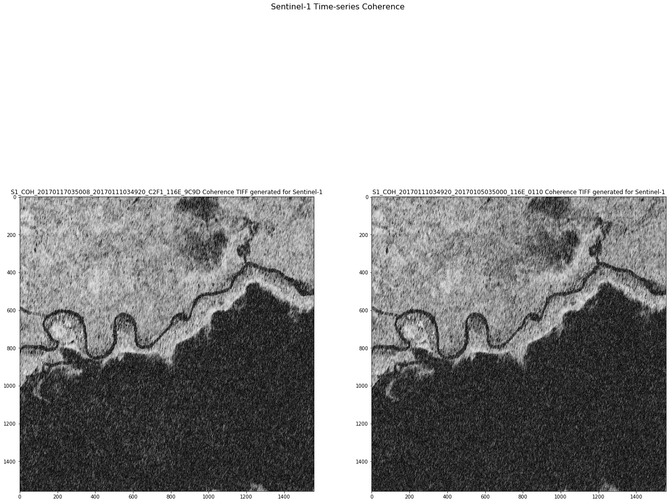
['S1_COH_20170117035008_20170111034920_C2F1_116E_9C9D Coherence TIFF generated for Sentinel-1', 'S1_COH_20170111034920_20170105035000_116E_0110 Coherence TIFF generated for Sentinel-1']
In [20]:
bands[0]
Out[20]:
array([[ 118.11617862,  146.95844237,  163.98082921, ...,  154.07888524,
         151.71111947,  130.8025825 ],
       [ 123.23127122,  154.22944204,  165.680433  , ...,  149.85698784,
         162.48033789,  156.3873502 ],
       [ 130.03115798,  154.62673261,  170.3346128 , ...,  151.18214621,
         172.10005793,  177.36175966],
       ...,
       [  50.80664413,   66.29311177,   60.97882884, ...,  133.23751331,
         119.83819929,   86.2743649 ],
       [  73.2001153 ,   54.18494146,   57.58253337, ...,  130.09727963,
         117.61936297,   83.06476267],
       [  81.98398658,   48.50116524,   50.11064595, ...,  127.16311942,
         117.5535917 ,   91.37683584]])
In [27]:
fig = plt.figure(figsize=(20,20))

fig.suptitle('Sentinel-1 Time-series Coherence', fontsize=16)

for i in range(numbands):

    a = fig.add_subplot(1, numbands, i+1)

    imgplot = plt.imshow(bands[i].astype(np.uint8),
                         cmap='gray')
    a.set_title(titles[i])

plt.tight_layout()
fig = plt.gcf()
plt.show()

fig.clf()
plt.close()
Download functionalities
Download a product
- Define the download function
In [22]:
def get_product(url, dest, api_key):

    request_headers = {'X-JFrog-Art-Api': api_key}

    r = requests.get(url, headers=request_headers)

    open(dest, 'wb').write(r.content)

    return r.status_code
- Get the reference download endpoint for the product related to the first date
In [ ]:
enclosure = myGDF[(myGDF['startdate'] == mydates[0])]['enclosure'].values[0]

enclosure
In [ ]:
output_name = myGDF[(myGDF['startdate'] == mydates[0])]['title'].values[0]

output_name
In [ ]:
get_product(enclosure,
            output_name,
            api_key)
Bulk Download
- Define the bulk download function
In [ ]:
def get_product_bulk(row, api_key):

    return get_product(row['enclosure'],
                       row['title'],
                       api_key)
- Download all the products related to the chosen dates
In [ ]:
myGDF.apply(lambda row: get_product_bulk(row, api_key), axis=1)