better-wfp-00004 data pipeline results (Landsat 8 reflectances and vegetation indices) : metadata loading from pickle file and results exploiting
This Notebook shows how: * to re-load better-wfp-00004 data pipeline results previously stored in a pickle file * Create a new dataframe with data values cropped over the area of interest * Plot an RGB * Create a geotif
Import needed modules
In [1]:
import pandas as pd
from geopandas import GeoDataFrame
import gdal
import numpy as np
from shapely.geometry import Point
from shapely.geometry import Polygon
import matplotlib
import matplotlib.pyplot as plt
from PIL import Image
%matplotlib inline
from shapely.wkt import loads
from shapely.geometry import box
from urlparse import urlparse
import requests
Read picke data file
In [2]:
pickle_filename = 'better-wfp-00004_Sep_2017_Afghanistan.pkl'
- Create the data frame from the pickle file
In [3]:
results = GeoDataFrame(pd.read_pickle(pickle_filename))
In [4]:
results.head()
Out[4]:
| enclosure | enddate | identifier | self | startdate | title | |
|---|---|---|---|---|---|---|
| 0 | https://store.terradue.com/better-wfp-00004/_r... | 2017-09-30 06:00:36.979 | 9980cc8e1efcf19ae634102f03c06ceba5edaf39 | https://catalog.terradue.com//better-wfp-00004... | 2017-09-30 06:00:05.209 | Reproducibility stage-in notebook for Landsat8... |
| 1 | https://store.terradue.com/better-wfp-00004/_r... | 2017-09-30 06:00:36.979 | b1fe92b3e2bf685e3b191fa0c1a854f47d610ff9 | https://catalog.terradue.com//better-wfp-00004... | 2017-09-30 06:00:05.209 | Reproducibility notebook used for generating L... |
| 2 | https://store.terradue.com/better-wfp-00004/_r... | 2017-09-30 06:00:36.979 | 18a24ef01b5428b839d530a68c15261834ef1ad6 | https://catalog.terradue.com//better-wfp-00004... | 2017-09-30 06:00:05.209 | LC08_L1TP_153035_20170930_20171013_01_T1_R5.TIF |
| 3 | https://store.terradue.com/better-wfp-00004/_r... | 2017-09-30 06:00:36.979 | 266cdb8f2a06c0bfe50d564f17b7037d21e0088f | https://catalog.terradue.com//better-wfp-00004... | 2017-09-30 06:00:05.209 | LC08_L1TP_153035_20170930_20171013_01_T1_R2.TIF |
| 4 | https://store.terradue.com/better-wfp-00004/_r... | 2017-09-30 06:00:36.979 | 4f6a147dff6f11aa6bbcecea794c35ffefbe8a76 | https://catalog.terradue.com//better-wfp-00004... | 2017-09-30 06:00:05.209 | LC08_L1TP_153035_20170930_20171013_01_T1_R6.TIF |
Time of interest
In [5]:
mydate = '2017-09-21 06:06:12.098'
Area of interest
- The user can choose to define an AOI selecting a Point and a buffer size used to build a squared polygon around that point
In [6]:
point_of_interest = Point(67.890, 36.182)
In [7]:
buffer_size = 0.05
In [8]:
aoi_wkt = box(*point_of_interest.buffer(buffer_size).bounds)
In [9]:
aoi_wkt.wkt
Out[9]:
'POLYGON ((67.94 36.13200000000001, 67.94 36.232, 67.84 36.232, 67.84 36.13200000000001, 67.94 36.13200000000001))'
- Or create a Polygon from a points list (in this case this is exactly the Afghanistan reference AOI)
In [71]:
aoi_wkt = Polygon([(67.62430000000001, 36.7228), (68.116, 36.7228), (68.116, 35.6923), (67.62430000000001, 35.6923), (67.62430000000001, 36.7228)])
In [72]:
aoi_wkt.wkt
Out[72]:
'POLYGON ((67.62430000000001 36.7228, 68.116 36.7228, 68.116 35.6923, 67.62430000000001 35.6923, 67.62430000000001 36.7228))'
Provide here your ellip username and api key for platform access
In [10]:
import getpass

user = getpass.getpass("Enter your username:")
api_key = getpass.getpass("Enter the API key:")
Define 2 auxiliary methods to add data to the dataframe
- The first one gets single band data from url as array
In [11]:
def get_cropped_image_as_array(url, bbox):

    #[-projwin ulx uly lrx lry]
    ulx, uly, lrx, lry = bbox[0], bbox[3], bbox[2], bbox[1]

    output = '/vsimem/clip.tif'

    ds = gdal.Open('/vsicurl/%s' % url)
    ds = gdal.Translate(output, ds, projWin = [ulx, uly, lrx, lry], projWinSRS = 'EPSG:4326')
    ds = None

    ds = gdal.Open('/vsimem/clip.tif')
    band = ds.GetRasterBand(1)

    w = band.XSize
    h = band.YSize

    data = band.ReadAsArray(0, 0, w, h).astype(np.float)

    data[data==-9999] = np.nan

    ds = None
    band = None

    return data
- The second one selects the bands to be managed (everything but RT and T1 bands), gets the cropped data (wrt a given AOI) and returns the related stack
In [12]:
def get_info(row, bbox, user, api_key):

    extended_info = dict()

    # add the band info
    extended_info['band'] = row['title'].rsplit('_', 1)[1].split('.')[0]
    print 'Managing %s' %row['title']
    # add the data for the AOI
    if not extended_info['band'] in ['RT', 'T1']:
        print 'Getting band %s' %extended_info['band']
        parsed_url = urlparse(row['enclosure'])

        url = '%s://%s:%s@%s/api%s' % (list(parsed_url)[0], user, api_key, list(parsed_url)[1], list(parsed_url)[2])

        extended_info['aoi_data'] = get_cropped_image_as_array(url, bbox)

    # create the series
    series = pd.Series(extended_info)

    return series
Create a new dataframe with data values
- Select from metadataframe a subframe related to the time of interest
- Add to the subframe the related data values cropped with respect to the AOI bounds
In [13]:
mydate_results = results[(results['startdate'] == mydate) & (results.apply(lambda row: 'Reproducibility' not in row['title'], axis=1))]
mydate_results.head()
Out[13]:
| enclosure | enddate | identifier | self | startdate | title | |
|---|---|---|---|---|---|---|
| 18 | https://store.terradue.com/better-wfp-00004/_r... | 2017-09-21 06:06:43.868 | 9ac056edcf00d6293ce8fec76f6a03d09c8f0218 | https://catalog.terradue.com//better-wfp-00004... | 2017-09-21 06:06:12.098 | LC08_L1TP_154035_20170921_20171012_01_T1_R8.TIF |
| 19 | https://store.terradue.com/better-wfp-00004/_r... | 2017-09-21 06:06:43.868 | e74b529b44f575ab88511ec148880b17c76d4bbe | https://catalog.terradue.com//better-wfp-00004... | 2017-09-21 06:06:12.098 | LC08_L1TP_154035_20170921_20171012_01_T1_R9.TIF |
| 20 | https://store.terradue.com/better-wfp-00004/_r... | 2017-09-21 06:06:43.868 | 0a8eac9e73dc53e94a7bfc422860376c406d49db | https://catalog.terradue.com//better-wfp-00004... | 2017-09-21 06:06:12.098 | LC08_L1TP_154035_20170921_20171012_01_T1_R2.TIF |
| 21 | https://store.terradue.com/better-wfp-00004/_r... | 2017-09-21 06:06:43.868 | 21c0df06c92decfd7e5cab488e5b7ebd50a78466 | https://catalog.terradue.com//better-wfp-00004... | 2017-09-21 06:06:12.098 | LC08_L1TP_154035_20170921_20171012_01_T1_NDBI.TIF |
| 22 | https://store.terradue.com/better-wfp-00004/_r... | 2017-09-21 06:06:43.868 | 24dc75d1b8e9c39b3b51400e66f71049e8ed4cee | https://catalog.terradue.com//better-wfp-00004... | 2017-09-21 06:06:12.098 | LC08_L1TP_154035_20170921_20171012_01_T1_R3.TIF |
In [14]:
mydate_results = mydate_results.merge(mydate_results.apply(lambda row: get_info(row, list(aoi_wkt.bounds), user, api_key), axis=1), left_index=True, right_index=True)
Managing LC08_L1TP_154035_20170921_20171012_01_T1_R8.TIF
Getting band R8
Managing LC08_L1TP_154035_20170921_20171012_01_T1_R9.TIF
Getting band R9
Managing LC08_L1TP_154035_20170921_20171012_01_T1_R2.TIF
Getting band R2
Managing LC08_L1TP_154035_20170921_20171012_01_T1_NDBI.TIF
Getting band NDBI
Managing LC08_L1TP_154035_20170921_20171012_01_T1_R3.TIF
Getting band R3
Managing LC08_L1TP_154035_20170921_20171012_01_T1_R1.TIF
Getting band R1
Managing LC08_L1TP_154035_20170921_20171012_01_T1_MNDWI.TIF
Getting band MNDWI
Managing LC08_L1TP_154035_20170921_20171012_01_T1_NDVI.TIF
Getting band NDVI
Managing LC08_L1TP_154035_20170921_20171012_01_T1_R6.TIF
Getting band R6
Managing LC08_L1TP_154035_20170921_20171012_01_T1_NDWI.TIF
Getting band NDWI
Managing LC08_L1TP_154035_20170921_20171012_01_T1_R7.TIF
Getting band R7
Managing LC08_L1TP_154035_20170921_20171012_01_T1_R4.TIF
Getting band R4
Managing LC08_L1TP_154035_20170921_20171012_01_T1_BQA.TIF
Getting band BQA
Managing LC08_L1TP_154035_20170921_20171012_01_T1_R5.TIF
Getting band R5
In [15]:
mydate_results.head()
Out[15]:
| enclosure | enddate | identifier | self | startdate | title | aoi_data | band | |
|---|---|---|---|---|---|---|---|---|
| 18 | https://store.terradue.com/better-wfp-00004/_r... | 2017-09-21 06:06:43.868 | 9ac056edcf00d6293ce8fec76f6a03d09c8f0218 | https://catalog.terradue.com//better-wfp-00004... | 2017-09-21 06:06:12.098 | LC08_L1TP_154035_20170921_20171012_01_T1_R8.TIF | [[0.194399997592, 0.173600003123, 0.1584800034... | R8 |
| 19 | https://store.terradue.com/better-wfp-00004/_r... | 2017-09-21 06:06:43.868 | e74b529b44f575ab88511ec148880b17c76d4bbe | https://catalog.terradue.com//better-wfp-00004... | 2017-09-21 06:06:12.098 | LC08_L1TP_154035_20170921_20171012_01_T1_R9.TIF | [[0.0048600002192, 0.00449999980628, 0.0044599... | R9 |
| 20 | https://store.terradue.com/better-wfp-00004/_r... | 2017-09-21 06:06:43.868 | 0a8eac9e73dc53e94a7bfc422860376c406d49db | https://catalog.terradue.com//better-wfp-00004... | 2017-09-21 06:06:12.098 | LC08_L1TP_154035_20170921_20171012_01_T1_R2.TIF | [[0.151920005679, 0.140719994903, 0.1329600065... | R2 |
| 21 | https://store.terradue.com/better-wfp-00004/_r... | 2017-09-21 06:06:43.868 | 21c0df06c92decfd7e5cab488e5b7ebd50a78466 | https://catalog.terradue.com//better-wfp-00004... | 2017-09-21 06:06:12.098 | LC08_L1TP_154035_20170921_20171012_01_T1_NDBI.TIF | [[0.0651060193777, 0.0775961130857, 0.05901997... | NDBI |
| 22 | https://store.terradue.com/better-wfp-00004/_r... | 2017-09-21 06:06:43.868 | 24dc75d1b8e9c39b3b51400e66f71049e8ed4cee | https://catalog.terradue.com//better-wfp-00004... | 2017-09-21 06:06:12.098 | LC08_L1TP_154035_20170921_20171012_01_T1_R3.TIF | [[0.173460006714, 0.157299995422, 0.1448200047... | R3 |
- Show data values of NDVI bands
In [16]:
list(mydate_results[mydate_results['band'] == 'NDVI']['aoi_data'].values)
Out[16]:
[array([[ 0.12459698,  0.12829348,  0.13730125, ...,  0.13223022,
          0.12330148,  0.12979481],
        [ 0.12104059,  0.12093267,  0.12302252, ...,  0.12557122,
          0.13161042,  0.12638074],
        [ 0.11792592,  0.12007882,  0.11558118, ...,  0.12352817,
          0.11645769,  0.112569  ],
        ...,
        [ 0.13985506,  0.13362254,  0.13503377, ...,  0.16269179,
          0.16708173,  0.1453025 ],
        [ 0.13852298,  0.13686992,  0.13524064, ...,  0.16952896,
          0.18446405,  0.16196381],
        [ 0.14452948,  0.14335296,  0.13800251, ...,  0.1733848 ,
          0.17413892,  0.17204562]])]
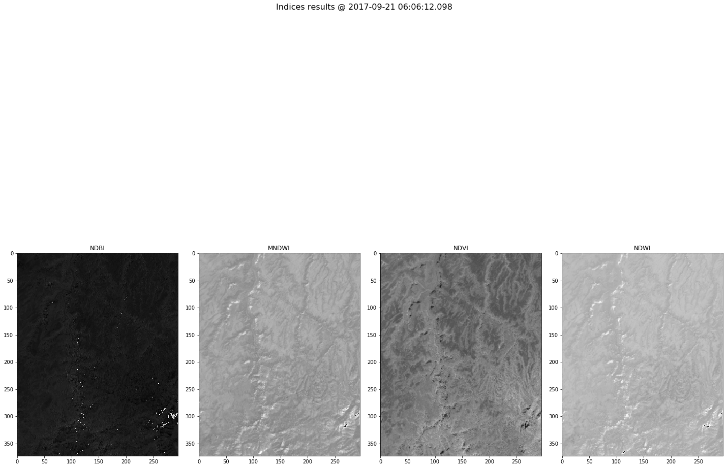
Plot functionality
- Plot vegetation indices of the selected result
In [17]:
indices_bands=mydate_results[(mydate_results['band'] == 'NDVI') |
                             (mydate_results['band'] == 'NDWI') |
                             (mydate_results['band'] == 'NDBI') |
                             (mydate_results['band'] == 'MNDWI')]

num_bands = len(indices_bands)
In [18]:
min_reflec = 0.2
max_reflec = 1.0


fig = plt.figure(figsize=(20,20))

fig.suptitle('Indices results @ %s' % (mydate), fontsize=16)

for i,row in enumerate(indices_bands.iterrows()):
    band = row[1]['aoi_data']
    band = band * 255 / (max_reflec - min_reflec)
    a = fig.add_subplot(1, num_bands, i+1)

    imgplot = plt.imshow(band.astype(np.uint8),
                         cmap='gray')
    a.set_title(row[1]['band'])

plt.tight_layout()
fig = plt.gcf()
plt.show()

fig.clf()
plt.close()
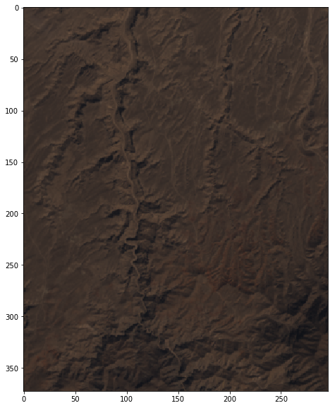
- Plot an RGB
Choosing a reference day to plot data
In [19]:
band_red = mydate_results[(mydate_results['band'] == 'R4')]['aoi_data'].values[0]
band_green = mydate_results[(mydate_results['band'] == 'R3')]['aoi_data'].values[0]
band_blue = mydate_results[(mydate_results['band'] == 'R2')]['aoi_data'].values[0]
In [20]:
min_reflec = 0.2
max_reflec = 1.0

bands = [(band_red * 255 / (max_reflec - min_reflec)),
         (band_green * 255 / (max_reflec - min_reflec)),
         (band_blue * 255 / (max_reflec - min_reflec))]
In [21]:
rgb_uint8 = np.dstack(bands).astype(np.uint8)

width = 10
height = 10
plt.figure(figsize=(width, height))
img = Image.fromarray(rgb_uint8)
imgplot = plt.imshow(img)
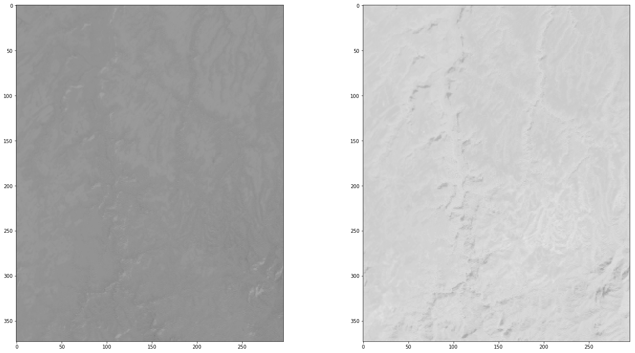
Create a geotif with the area of interest
In [22]:
parsed_url = urlparse(mydate_results[(mydate_results['band'] == 'R4')]['enclosure'].values[0])
In [23]:
ulx, uly, lrx, lry = aoi_wkt.bounds

output = '/vsimem/clip.tif'

ds = gdal.Open('/vsicurl/%s://%s:%s@%s/api%s' % (list(parsed_url)[0], user, api_key, list(parsed_url)[1], list(parsed_url)[2]))
ds = gdal.Translate(output, ds, projWin = [ulx, uly, lrx, lry], projWinSRS = 'EPSG:4326')
ds = None

ds = gdal.Open(output)
geo_transform = ds.GetGeoTransform()
projection = ds.GetProjection()

band = ds.GetRasterBand(1)

cols = band.XSize
rows = band.YSize
In [24]:
geo_transform
Out[24]:
(395745.0, 30.0, 0.0, 4010325.0, 0.0, -30.0)
In [25]:
projection
Out[25]:
'PROJCS["WGS 84 / UTM zone 42N",GEOGCS["WGS 84",DATUM["WGS_1984",SPHEROID["WGS 84",6378137,298.257223563,AUTHORITY["EPSG","7030"]],AUTHORITY["EPSG","6326"]],PRIMEM["Greenwich",0,AUTHORITY["EPSG","8901"]],UNIT["degree",0.0174532925199433,AUTHORITY["EPSG","9122"]],AUTHORITY["EPSG","4326"]],PROJECTION["Transverse_Mercator"],PARAMETER["latitude_of_origin",0],PARAMETER["central_meridian",69],PARAMETER["scale_factor",0.9996],PARAMETER["false_easting",500000],PARAMETER["false_northing",0],UNIT["metre",1,AUTHORITY["EPSG","9001"]],AXIS["Easting",EAST],AXIS["Northing",NORTH],AUTHORITY["EPSG","32642"]]'
In [26]:
print(cols, rows)
(296, 373)
In [27]:
band1_data = mydate_results[(mydate_results['band'] == 'NDVI')]['aoi_data'].values[0]
band2_data = mydate_results[(mydate_results['band'] == 'NDWI')]['aoi_data'].values[0]
In [28]:
band_number = 2

drv = gdal.GetDriverByName('GTiff')

ds = drv.Create('export.tif', cols, rows, band_number, gdal.GDT_Float32)

ds.SetGeoTransform(geo_transform)
ds.SetProjection(projection)

ds.GetRasterBand(1).WriteArray(band1_data, 0, 0)
ds.GetRasterBand(2).WriteArray(band2_data, 0, 0)
ds.FlushCache()
In [29]:
fig = plt.figure(figsize=(20,20))

for i in [0,1]:

    a=fig.add_subplot(2, 2, 0+i+1)

    imgplot = plt.imshow(ds.GetRasterBand(i+1).ReadAsArray().astype(np.float),
                         cmap=plt.cm.binary,
                         vmin=-0.5,
                         vmax=1)

plt.tight_layout()
fig = plt.gcf()
plt.show()

fig.clf()
plt.close()
In [30]:
mydate_results[mydate_results['band'] == 'NDVI']['self'].values
Out[30]:
array([ 'https://catalog.terradue.com//better-wfp-00004/series/results/search?format=atom&uid=57bbbfa9bc5339ac88d930e95acc7dd2a97df501'], dtype=object)
Download functionality
Single product download
In [32]:
def get_product(url, dest, api_key):

    request_headers = {'X-JFrog-Art-Api': api_key}

    r = requests.get(url, headers=request_headers)

    open(dest, 'wb').write(r.content)

    return r.status_code
- Select the bands to be downloaded
In [33]:
enclosure = mydate_results[(mydate_results['band'] == 'NDVI')]['enclosure'].values[0]

enclosure
Out[33]:
'https://store.terradue.com/better-wfp-00004/_results/workflows/ec_better_ewf_wfp_01_02_02_ewf_wfp_01_02_02_0_11/run/a4af56da-27b3-11e9-962c-0242ac11000f/0003156-181221095105003-oozie-oozi-W/30b20fe9-ebbe-4d1a-bd12-6b52b259187a/LC08_L1TP_154035_20170921_20171012_01_T1_NDVI.TIF'
In [34]:
output_name = mydate_results[(mydate_results['band'] == 'NDVI') ]['title'].values[0]

output_name
Out[34]:
'LC08_L1TP_154035_20170921_20171012_01_T1_NDVI.TIF'
In [35]:
get_product(enclosure,
            output_name,
            api_key)
Out[35]:
200
Bulk Download
In [36]:
def get_product_bulk(row, api_key):

    return get_product(row['enclosure'],
                       row['title'],
                       api_key)
- Bulk download of NDVI and NDBI bands
In [38]:
mydate_results[(mydate_results['band'] == 'NDVI') | (mydate_results['band'] == 'NDBI')].apply(lambda row: get_product_bulk(row, api_key), axis=1)
Out[38]:
18    200
19    200
20    200
21    200
22    200
23    200
24    200
25    200
26    200
27    200
28    200
29    200
30    200
31    200
dtype: int64
- Or download all the mydate results content
In [39]:
mydate_results.apply(lambda row: get_product_bulk(row, api_key), axis=1)
Out[39]:
18    200
19    200
20    200
21    200
22    200
23    200
24    200
25    200
26    200
27    200
28    200
29    200
30    200
31    200
dtype: int64