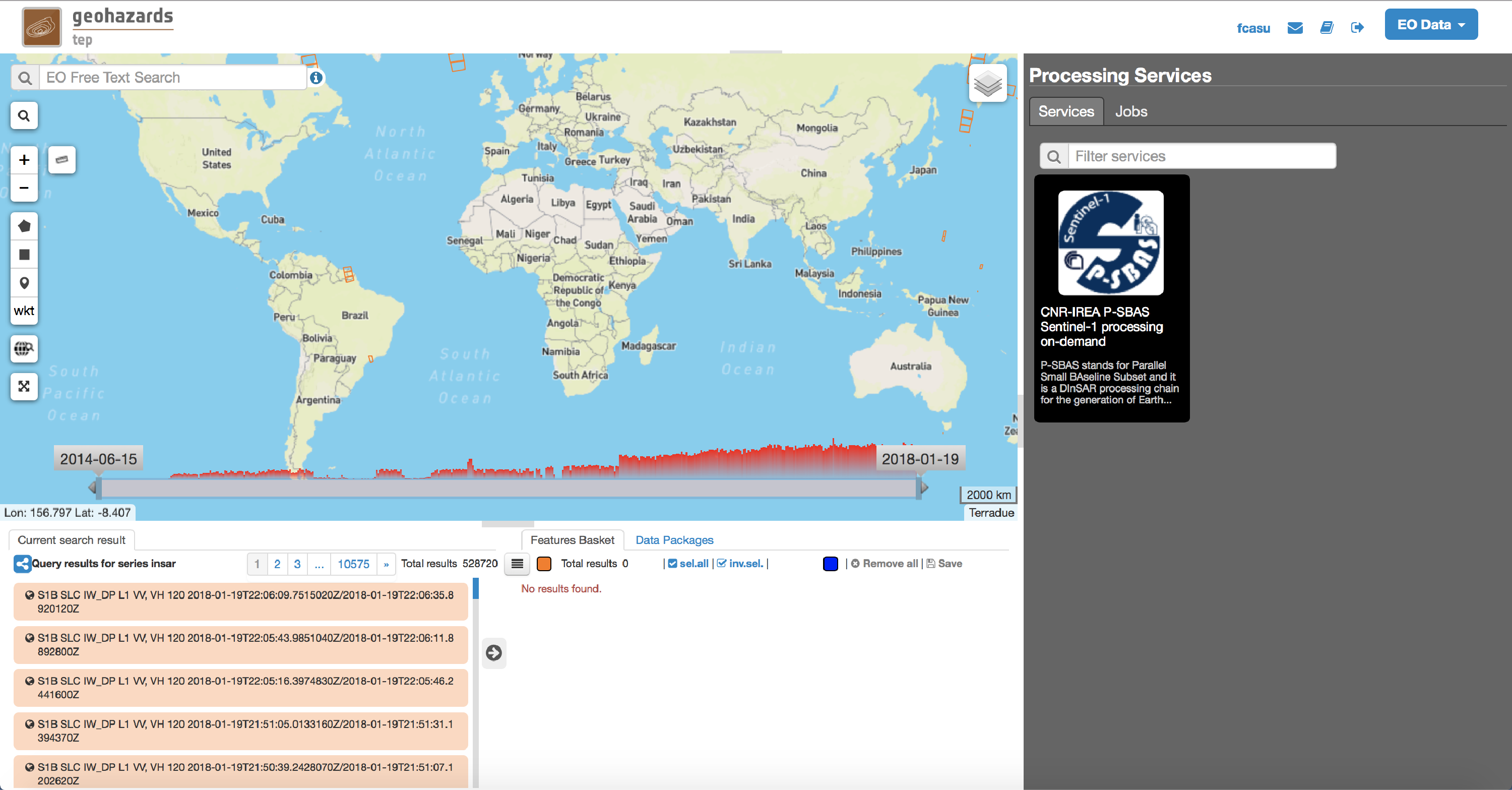
P-SBAS Sentinel-1 processing on-demand by CNR-IREA¶

P-SBAS InSAR Sentinel-1 TOPS (GEP)

P-SBAS stands for Parallel Small BAseline Subset and it is a DInSAR processing chain for the generation of Earth deformation time series and mean velocity maps. Input: SLC (Level-1) Sentinel-1 data. Output: LOS Displacement time series; Mean LOS Velocity; Temporal Coherence; Average scatterer elevation (Topography). Output Format: CSV. (The service can also generate wrapped and unwrapped interferograms that are delivered in geoTiff format).

EO sources supported:

Sentinel-1 TOPSAR IW SLC

Output specifications

(Default) LOS Displacement time series; Mean LOS Velocity; Temporal Coherence; Average scatterer elevation (Topography). Format: CSV.

(Upon request) Wrapped Interferograms; Unwrapped Interferograms; Spatial coherence; Map of LOS vector. Format: GeoTIFF.

This tutorial describes how to submit a job for the CNR-IREA P-SBAS Sentinel-1 (S1) processing on-demand service to obtain a ground displacement time series from S1 SLAC (Level-1) data. P-SBAS stands for Parallel Small BAseline Subset and it is a DInSAR processing chain for the generation of Earth deformation time series and mean velocity maps The tutorial is addressed to users already familiar with InSAR processing, analysis and products, and gives some hints and recommendation for the best service usage experience.

The provided service performs the full P-SBAS DInSAR chain from SLC data (Level 1) retrieval to displacement time series generation, upon the Multi Temporal Analysis (MTA) processing mode.

The main user actions are the following:

select the Input SAR SLC data to be processed;
optionally define the area of SAR data to be processed;
set input parameters/threshold (e.g. reference point, polarization, …) for P-SBAS DInSAR processing;
obtain P-SBAS DInSAR geocoded (Lat/Lon WGS84) results, such as: LOS Displacement time series; Mean LOS Velocity; Temporal Coherence; Average scatterer elevation (Topography).

As additional feature, the possibility to generate single or stack of interferograms co-registered to a single master geometry is also available, within the Interferogram Generation (IFG) processing mode.

Users are encouraged to use the P-SBAS DInSAR service here described for scientific purposes. The results (including products, maps, time series, files and everything generated by the processors) of the service are available under the CC-BY license. See “Terms and Conditions” section below for more details. Accordingly, please recognize the effort made by the authors by citing:

Casu, F., Elefante, E., Imperatore, P., Zinno, I., Manunta, M., De Luca, C., Lanari, R. (2014) “SBAS-DInSAR Parallel Processing for Deformation Time Series Computation”, IEEE JSTARS, doi: 10.1109/JSTARS.2014.2322671

Manunta, M., De Luca, C., Zinno I., Casu, F., Manzo, M., Bonano, M., Fusco, A., Pepe, A., Onorato, G., Berardino, P., De Martino, P., Lanari, R. (2019) “The Parallel SBAS Approach for Sentinel-1 Interferometric Wide Swath Deformation Time-Series Generation: Algorithm Description and Products Quality Assessment”, IEEE Trans. Geosci. Remote Sens., doi: 10.1109/TGRS.2019.2904912

De Luca, C., Cuccu, R., Elefante, S., Zinno, I., Manunta, M., Casola, V., Rivolta, G., Lanari, R., Casu, F. (2015) “An On-Demand Web Tool for the Unsupervised Retrieval of Earth’s Surface Deformation from SAR Data: The P-SBAS Service within the ESA G-POD Environment”, Remote Sens. 2015, 7(11), 15630-15650; doi:10.3390/rs71115630

in relevant talks, documents and publications prepared by using P-SBAS DInSAR results generated by this service. CNR-IREA and ESA do not respond in any case for the use, interpretation, and quality of the obtained measurements.

In the following, two service runs related to the two different processing modes (MTA and IFG) are provided.

1 Multi Temporal Analysis (MTA) Mode¶

1.1 Select the processing¶

Sign-in on the Portal https://geohazards-tep.eu/
Access the “CNR IREA SBAS Ground Motion Services” Thematic App.
Open the tab “Processing services” from the right of the map, and then select the processing service “CNR-IREA P-SBAS Sentinel-1 processing on-demand”.

1.2 Select the files to process¶

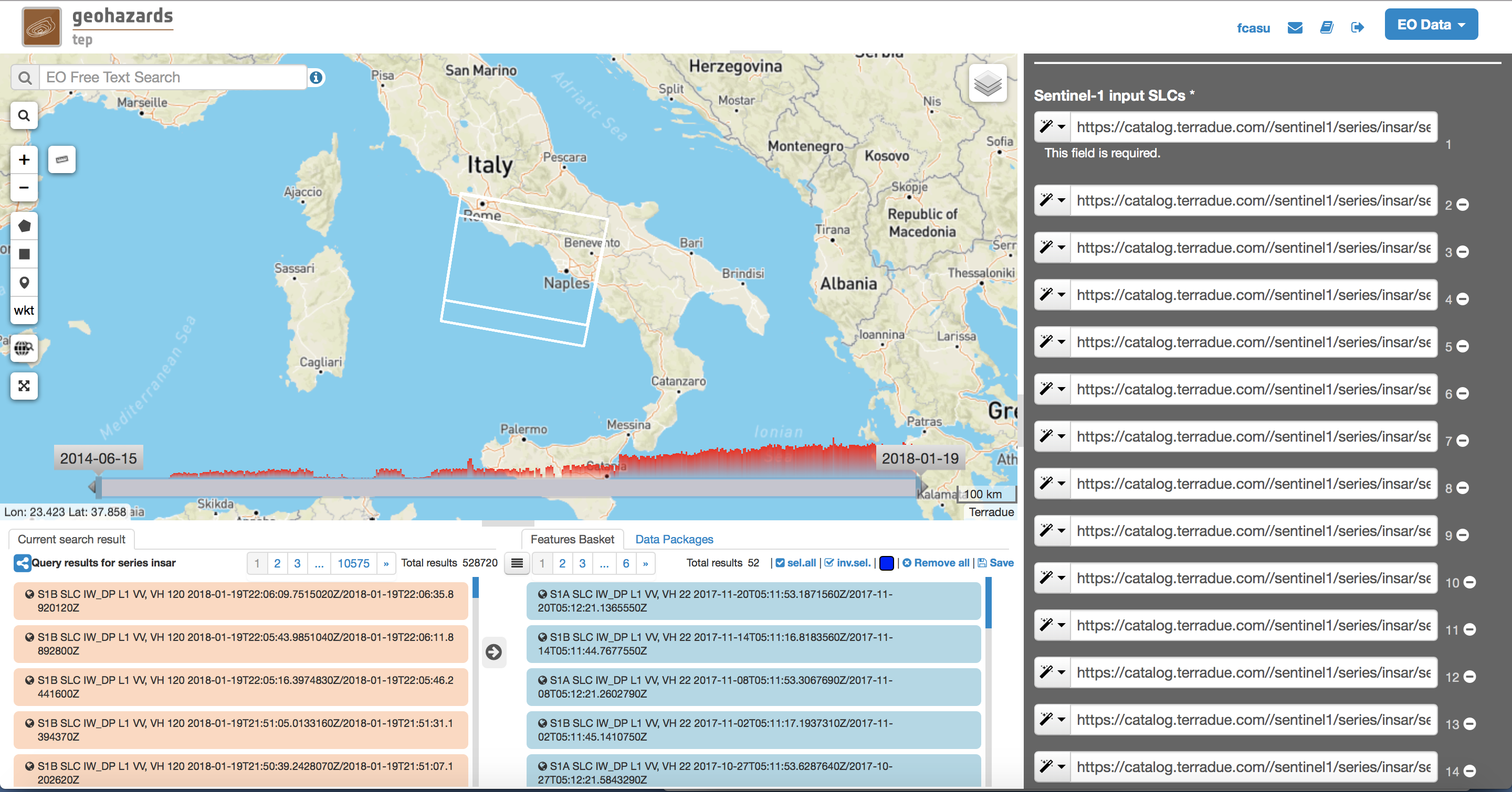
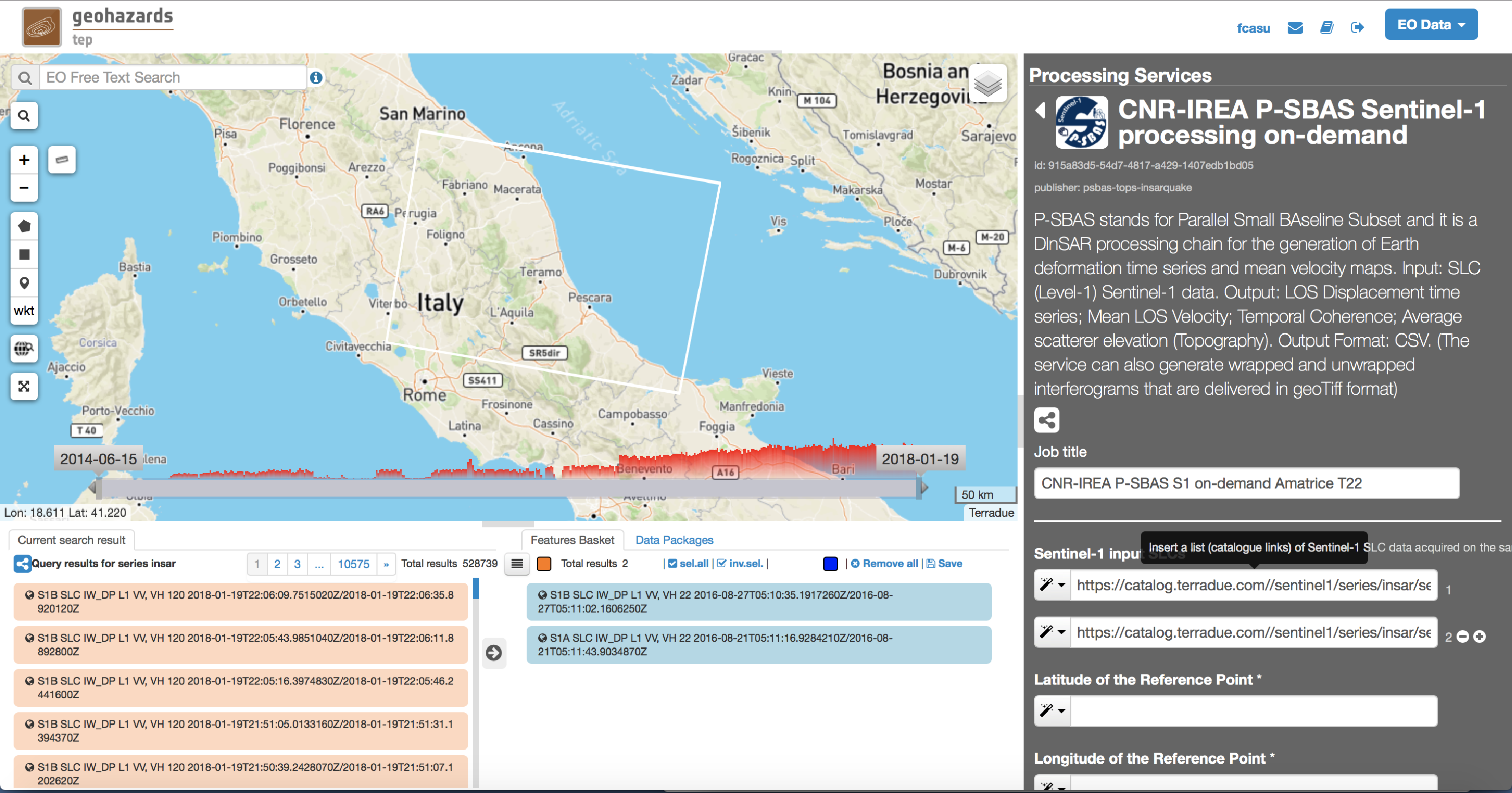
Input SAR data selection must be carried out with particular care, since a wrong data selection can result to an unfeasible processing.

The algorithm accepts as inputs IW Sentinel-1 SLC (level 1) data. RAW data cannot be processed.
It is very important that the user selects images related to the same track only which must be aquired with the same mode (the IW one).
The system automatically discards duplicated (reprocessed) images and correctly mosaicks SAR data belonging to different “portions” (slices) of the same strip. In case of reprocessed (duplicated) images the newest one is selected.
Note that to obtain reliable displacement measurements and to avoid processing failures, it is strongly suggested to select a number of epochs greater then 20 in the case of time series generation mode.

Note

Jobs submitted with less than 15 images in MTA mode will be automatically transformed into the IFG mode.

Note

The user should avoid temporal gaps larger than one year in the data set selection.

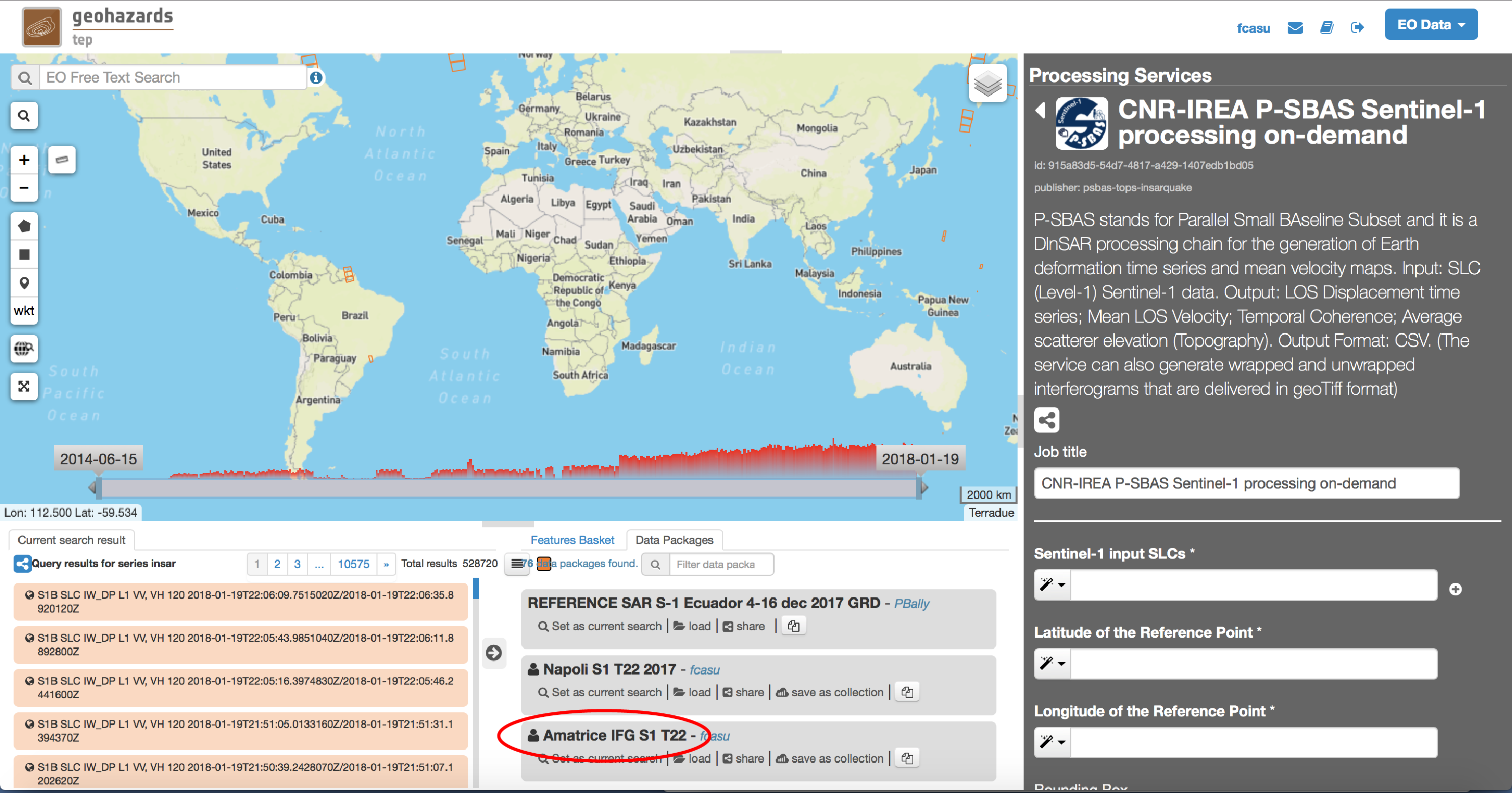
For this tutorial, a pre-defined data set has been prepared to speed up the data selection step .

Browse the Data Packages looking for Napoli S1 T22 2017 package and click on the load button to upload it.

Surf the map to the Napoli (Italy) Area of Interest: the browser page should appear as depicted in the next figure.

Set the Job Title with a meaningful name (e.g. CNR-IREA P-SBAS S1 Napoli T22 2017 - v1.0.9) and push the sel. all button in the Feature Basket.

Drag all the selected data and drop them within the Sentinel-1 input SLCs field on the right panel.

1.3 Fill the parameter values¶

Fill the parameters according to the following figure:

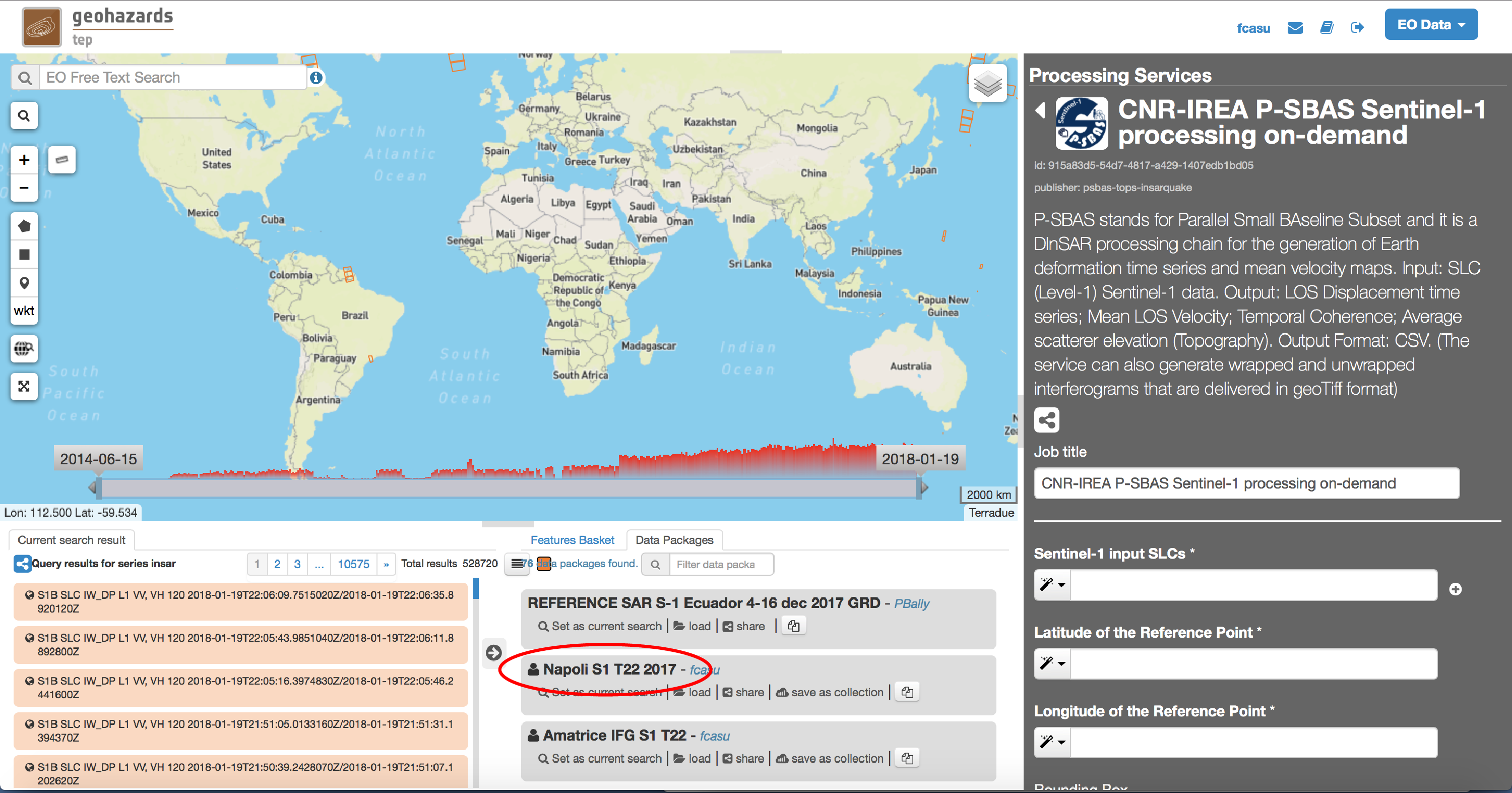
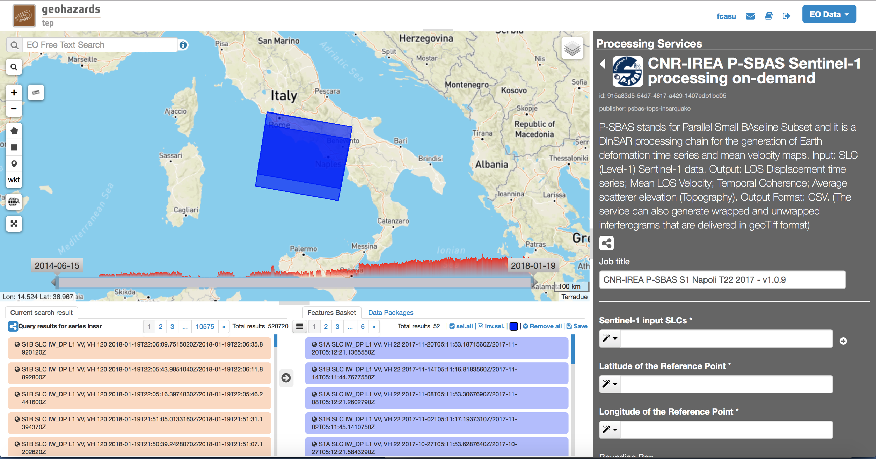
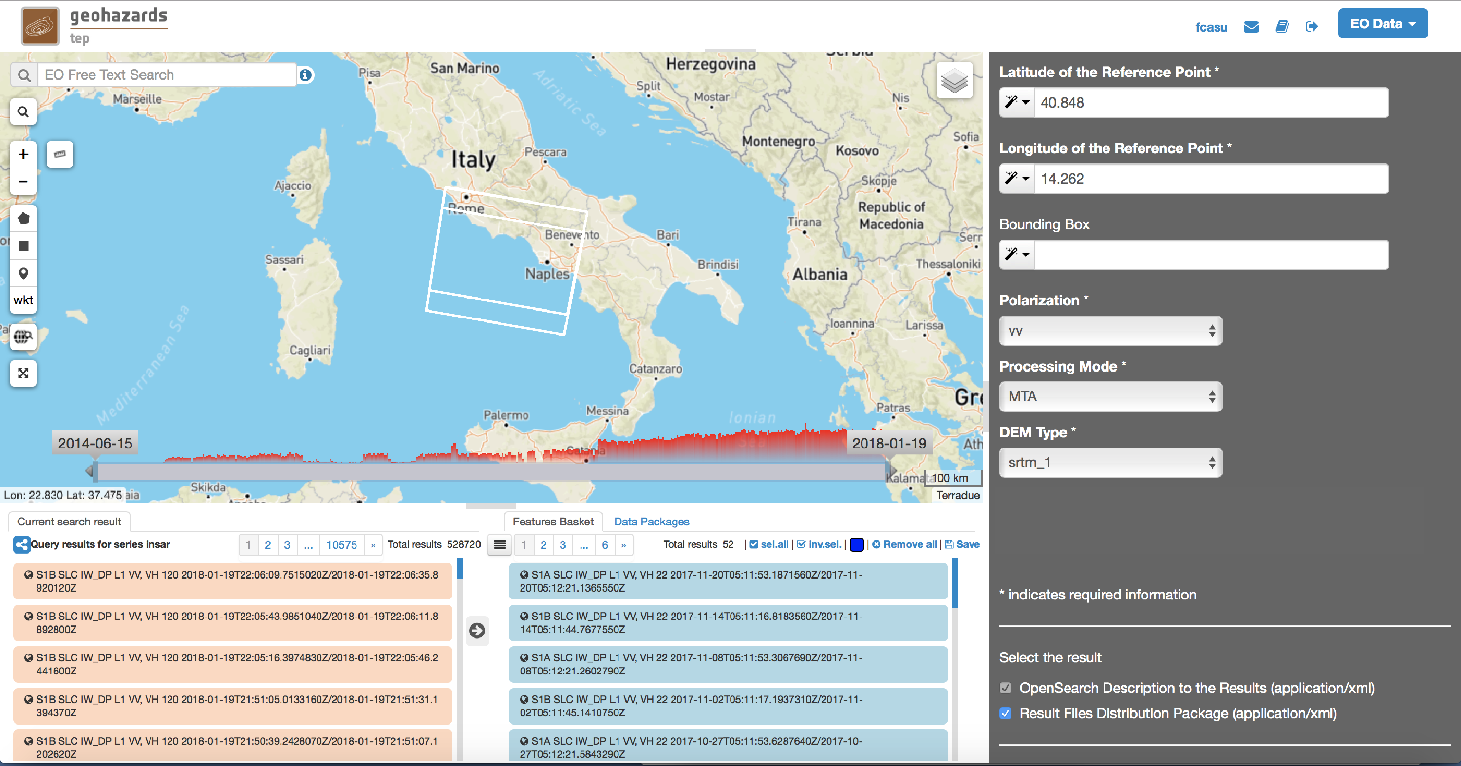
In particular:

As Latitude of the Reference Point, type:

40.848

As Longitude of the Reference Point, type:

14.262

Note

Latitude of the Reference Point and Longitude of the Reference Point are the Latitude and Longitude coordinates (in decimal degrees) of the reference point for the P-SBAS DInSAR measurement. It should be located in a stable area or its deformation behaviour shall be known. In any case, the user shall verify that input Latitude and Longitude coordinates are on land and included within the selected Area of Interest (if any, see next step). As a suggestion, urbanized areas are usually well suitable to locate the reference point. Moreover, it is in general a good practice to put the reference point in the deformation far field. The Magic Wand button can be used to automatically fill these fields with the coordinate values of a Marker placed on the map.

Note

To help the PhU, the algorithm automatically refines the reference point and selects the one with best coherence conditions close to the one selected by the user. This makes also the algorithm more robust to possible input mistakes. Moreover, at the end of the processing, the algorithm implements an average reference on the whole scene to avoid the dependance to one single point. This mitigates the effect of the reference point atmospheric noise, thus generating a sort of “absolute” reference to every zero-mean point. Anyway, the user can pick the time series of a point of interest and subtract it from the entire data set, so that the results are referred to a specific point.

Leave the Bounding Box untouched (Area of Interest empty).

Note

If set, the system automatically processes the identified AoI. Format: LL-Lon, LL-Lat, UR-Lon, UR-Lat. The Magic Wand button can be used to automatically fill this field with the bounding coordinate values of a rectangle drawn on the map. Different slices covering the AoI are automatically merged. It is recommended to avoid processing very small areas to allow the system to correctly estimate the co-registration shifts needed by the TOPS mode. The suggested smallest area spans at least 4 S1 bursts, which approximately corresponds to about 80 km along azimuth.

As Polarization type:

vv

Note

Possible values are: vv, vh, hv, hh. The user shall select the correct polarization according to the selected SLC input data. Default value is vv, being the default S1 polarization for data acquired over land.

As Processing Mode, select:

MTA

Note

Possible values: MTA (Multi-Temporal Analysis); IFG (Interferogram Generation). Default value is MTA. For IFG description see Section 2.

As DEM, select:

srtm_1

Note

SRTM valid in the [-56 deg, +60 deg] range of latitudes.

Note

Possible values are: srtm_1 (1 arcsec SRTM DEM), srtm_3 (3 arcsec SRTM DEM). User is kindly advised to check the EarthExplorer web site for actual data coverage.

Leave the Temporal Coherence Threshold unchanged.

Note

The threshold on the minimium allowed Temporal Coherence of each point can be set in the 0.7-0.9 range. By keeping in mind that every result should be properly validated, we recommend that only expert users modify the default value of this field.

1.4 Run the job¶

Click on the button “Run Job” at the bottom of the P-SBAS DInSAR processor tab, and monitor the progress of the running Job:
After about 48 hours of processing time, the job status should be “Success”.

1.5 Results: download and visualization¶

Download

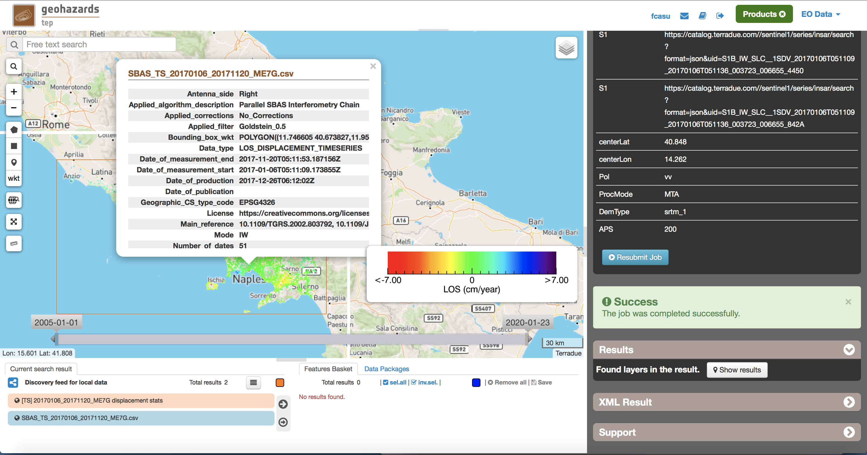
The P-SBAS DInSAR results are available in the Geobrowser after the processing. Scroll down the right panel and push the “Show results” button. Tutorial results are accessible here.

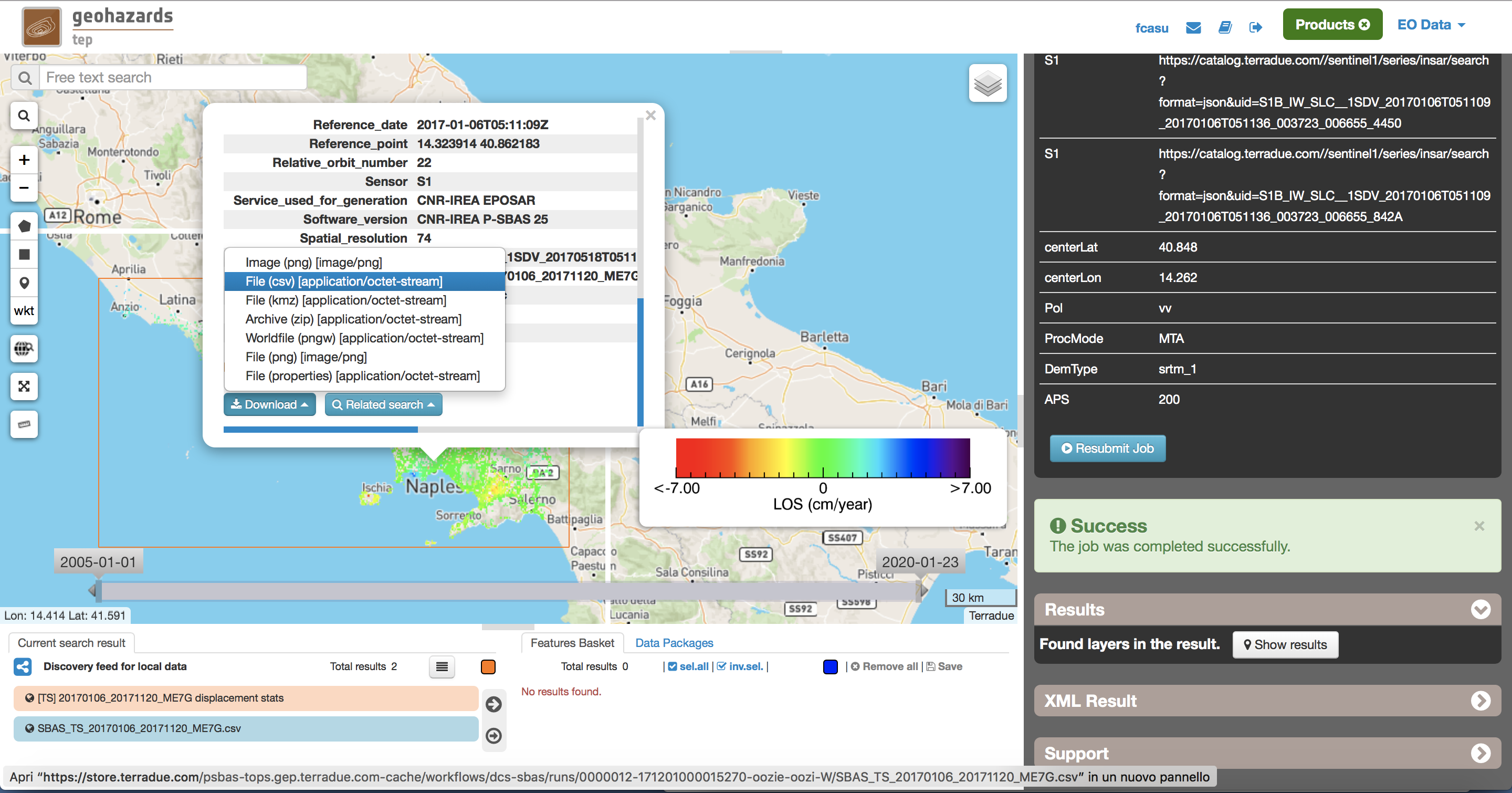
To download the P-SBAS DInSAR processing results once the Job is completed just click on the Download button in the pop-up window of the identified product:

Note

Single files can be downloaded separately. To download the full result archive, please select the zip file.

Visualization

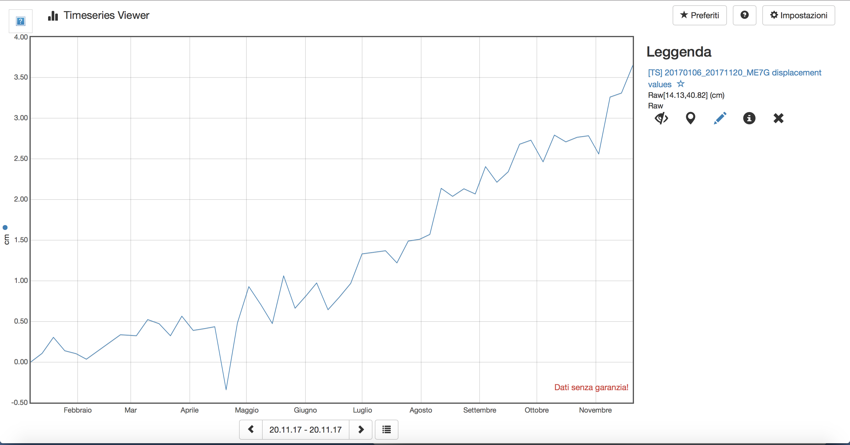
Time series can be directly visualized via the Geobrowser. After setting a satisfactory zoom, put a Placemark on the pixel for which the time series shold be displayed. Then click the “plot” icon in the TS collection.

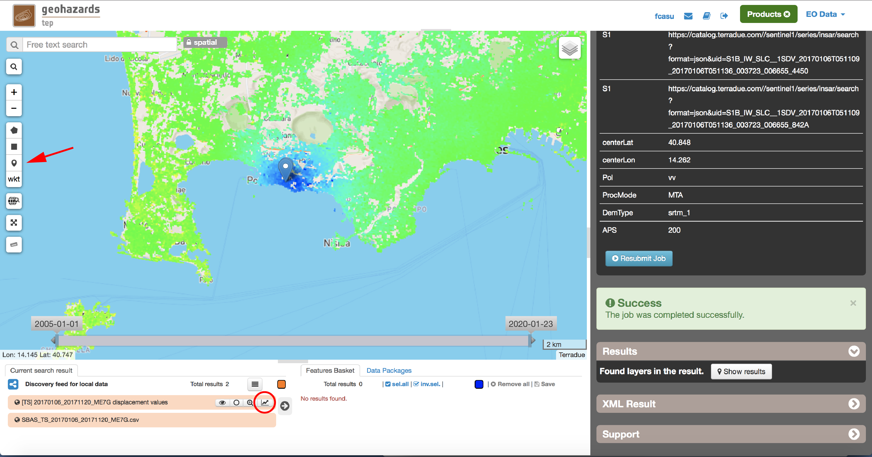
A pop-up window should appear showing the Time series of the selected pixel.

Conventions and assumptions

Results are provided in the satellite Line Of Sight (LOS). Positive values indicate that the target moves toward the satellite. Processing results are provided according to the EPOS-IP project specifications along with the corresponding metadata.

Published Results

The main outputs of the MTA mode are the:

Displacement Time series in LOS;
Mean LOS velocity;
Temporal coherence;
Pixel location (coordinates);
LOS unit vectors.

Information is organized in a CSV ASCII table according to the following figure.

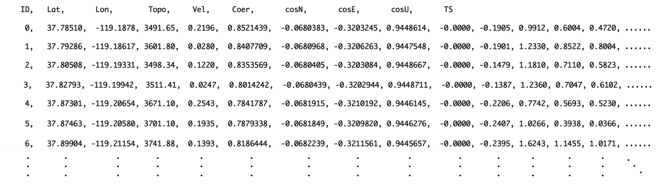
Provided information consists, per each pixel considered reliable, in:

Unique pixel identifier (ID);
WGS84 Latitude in degree (Lat);
WGS84 Longitude in degree (Lon);
Topography above the ellipsoid (Topo);
Mean Velocity in cm/year, as linear regression of the displacement Time series (Vel);
Temporal coherence (Coer);
Components of LOS unit vector along the North, East and Vertical directions (cosN, cosE, cosU);
LOS displacement time-series in cm (TS): the length of this field depends on the number of acquisitions used in the time series generation.

File name convention is as follows:

DTSLOS_<UserID>_<FirstAcqDate>_<LastAcqDate>_<UniqueCode>.csv

where:

<UserID> : is the name of the user or service that generated the product
<FirstAcqDate>: is the first acquisition of the time series;
<LastAcqDate> : is the last acquisition of the time series.
<UniqueCode> : is a unique code identifier.

A typical name sample is: DTSLOS_CNRIREA_20170106_20171120_ME7G.csv

Additional provided outputs are:

A .kmz file containing the Quick-look of the retrieved mean LOS velocity importable in Google Earth;
A .png file (together with its .pngw file) containing the raster bitmap image of the mean LOS velocity;
A .properties file containing the Metadata associated to the main results and displayed in the Geobrowser pop-up window;
A .png file representing the mean LOS velocity legend, i.e. the color code associated to the LOS Mean Velocity values;
A .zip archive that contains all the mentioned result files.

1.6 Metadata¶

Metadata are provided according to the EPOS specifications.

Tag	Example	Notes
Data_Type	LOS_DISPLACEMENT_TIMESERIES	Type of data (according to the EPOS categories)
Title	DTSLOS_CNRIREA_20170106_20171120_ME7G.csv	Title of the pop-up window (it corresponds to the file name)
Product_format	ASCII	Format of the product (geoTiff or CSV)
Product_size	23249970	In byte
Product_url		The url to locate the file
Bounding_box		The polygon relevant to the processed area
License	https://creativecommons.org/licenses/by/4.0	Applicable license for the product
User_ID	CNRIREA	User that generated the product
Software_version	CNR-IREA P-SBAS 25
Applied_algorithm_description	Parallel SBAS Interferometry Chain	Short description of the algorithm used to generate the product
Main_reference	10.1109/TGRS.2002.803792 10.1109/JSTARS.2014.232267	DOIs of the main publications describing the used algorithms
Date_of_measurement_start	2017-11-07T02:53:48.378740Z
Date_of_measurement_end	2017-11-19T02:53:48.215234Z
Date_of_production	2017-12-01T23:51:09Z
Date_of_publication	2017-12-01T23:51:09Z
Service_used_for_generation	EPOSAR
Geographic_CS_type_code	EPSG4326
Used_DEM	SRTM_3arcsec	DEM used within the interferometri processing
Super_master_SAR_image_ID	S1A_IW_SLC__1SDV_20171107T025348_20171107T025415_019153_02069A_D2C6.SAFE	Reference SAR geometry
Master_SAR_image_ID	S1A_IW_SLC__1SDV_20171107T025348_20171107T025415_019153_02069A_D2C6.SAFE	Master Image (only for IFG products)
Slave_SAR_image_ID	S1A_IW_SLC__1SDV_20171119T025348_20171119T025415_019328_020C14_14AF.SAFE	Slave Image (only for IFG products)
Perpendicular_baseline	-14.7667	In meters (only for IFG products)
Parallel_baseline	-4.35838	In meters (only for IFG products)
Along_track_baseline	-0.389812	In meters (only for IFG products)
Spatial_resolution	73	Ground resolution, in meters
Sensor	S1	Used sensor
Mode	IW	Acquisition mode
Antenna_side	Right	Right/Left
Relative_orbit_number	6	Satellite Track
Wavelength	0.055465760	In meters
Number_of_looks_azimuth	5	Applied multilook along azimuth
Number_of_looks_range	20	Applied multilook along range
Number_of_dates	51	Number of used acquisitions (only for MTA products)
Reference_date	2017-01-06T05:11:09Z	Acquisition used as temporal reference in the time series (only for MTA products)
Reference_point	14.323914 40.862183	Lon Lat format. For MTA and InU products
Applied_corrections	No_Corrections	Description of possible correction applied to the interferograms or time series
Applied_filter	Goldstein_0.5	Possible spatial filter applied to the interferogram

2 Interferogram Generation (IFG) Mode¶

2.1 Select the processing¶

Follow the steps described in Section 1.1.

2.2 Select the files to process¶

Input SAR data selection must be carried out with particular care, since a wrong data selection can result to an unfeasible processing.

The algorithm accepts as inputs IW Sentinel-1 SLC (level 1) data. RAW data cannot be processed.
It is very important that the user selects images related to the same track only which must be aquired with the same mode (the IW one).
The system automatically discards duplicated (reprocessed) images and correctly mosaicks SAR data belonging to different “portions” (slices) of the same strip. In case of reprocessed (duplicated) images the newest one is selected.

For this tutorial, a pre-defined data set has been prepared to speed up the data selection step.

Browse the Data Packages looking for Amatrice IFG S1 T22 package and click on the load button to upload it.

Surf the map to the Central Italy Area of Interest: the browser page should appear as depicted in the next figure.

Set the Job Title with a meaningful name (e.g. CNR-IREA P-SBAS S1 on-demand Amatrice T22) and push the sel. all button in the Feature Basket.
Drag all the selected data and drop them within the Sentinel-1 input SLCs field on the right panel.

2.3 Fill the parameter values¶

Fill the parameters according to the following figure:

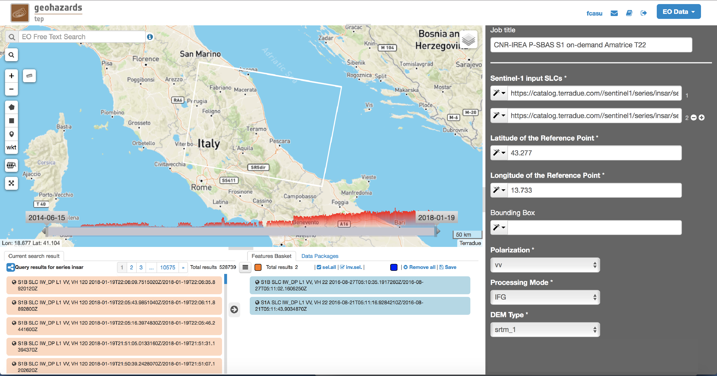
In particular:

As Latitude of the Reference Point, type:

43.277

As Longitude of the Reference Point, type:

13.733

Note

Leave the Bounding Box untouched (Area of Interest empty).

Note

Considerations as in Section 1.3 are valid.

As Polarization type:

vv

Note

As Processing Mode, select:

IFG

Note

Possible values: MTA (Multi-Temporal Analysis); IFG (Interferogram Generation). Default value is MTA. For MTA description see Section 1.

As DEM, select:

srtm_1

Note

SRTM valid in the [-56 deg, +60 deg] range of latitudes.

Note

Possible values are: srtm_1 (1 arcsec SRTM DEM), srtm_3 (3 arcsec SRTM DEM). User is kindly advised to check the EarthExplorer web site for actual data coverage.

2.4 Run the job¶

Click on the button “Run Job” at the bottom of the P-SBAS DInSAR processor tab, and monitor the progress of the running Job:
After about 4 hours of processing time, the job status should be as “Success”.

2.5 Results: download and visualization¶

The P-SBAS DInSAR results are available in the Geobrowser after the processing. Scroll down the right panel and push the “Show results” button. Tutorial results are accessible here.

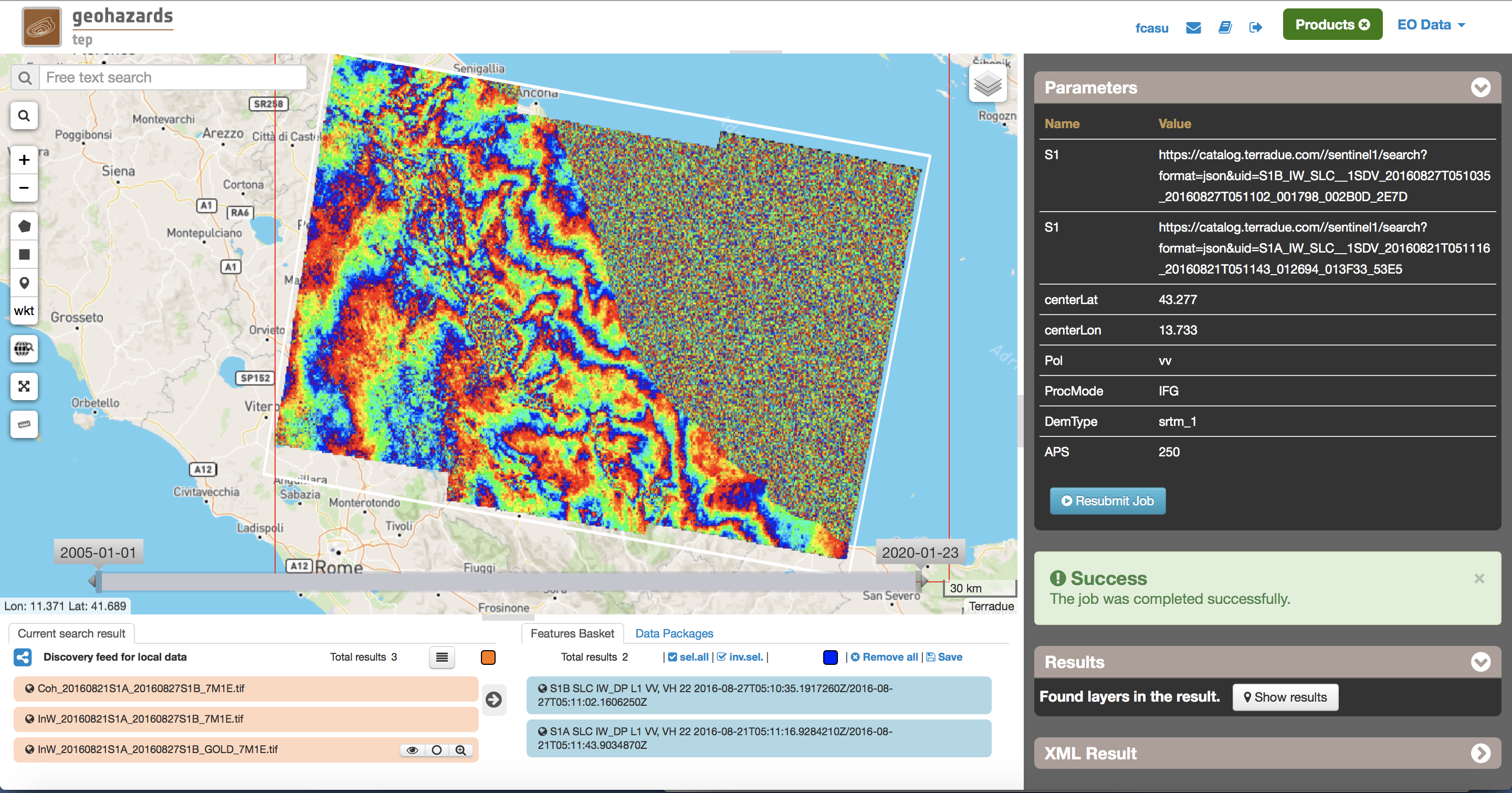
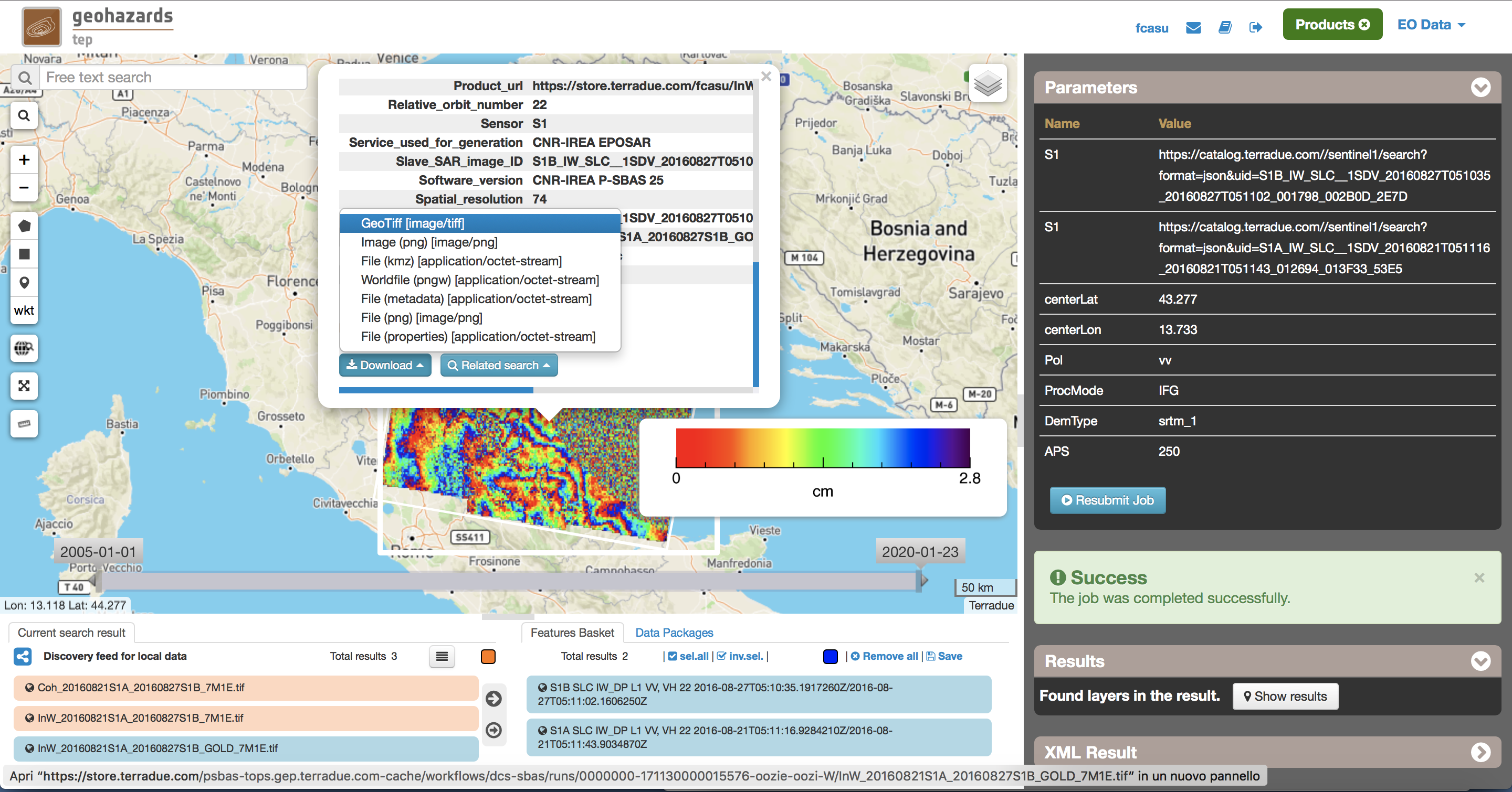
To download the P-SBAS DInSAR processing results once the Job is completed just click on the Download button in the pop-ip window of the identified product:

Conventions and assumptions

Published Results

The IFG mode outputs are provided in geoTiff standard and consist in:

geocoded interferograms (filtered and not filtered according to the Goldstein method);
geocoded spatial coherence maps.

The spacing of the output depends on the DEM used for the processing. Results are provided in WGS84 geographic projection.

File name convention is as follows:

<DataType>_<UserID>_<MasterDate>_<SlaveDate>_<UniqueCode>.<FileExtension>

where:

<DataType> can be: InW (Wrapped Interferogram), InU (Unwrapped Interferogram) (this feature will be available in a later release of the service), Coh (Spatial Coherence);
<UserID is the name of the user or service that generated the product;
<MasterDate> date of the Master acquisition in the format <yyyymmdd><SensorCode>, where <SensorCode> is a 3-char code that identifies the sensor. For the Sentinel case the possible codes are: S1A and S1B.
<SlaveDate> date of the Slave acquisition in the same <MasterDate> format;
<UniqueCode> a unique code identifier;
<FileExtension> possible values are:
- tif: the actual data in geoTiff;
- properties: the metadata displayed in the Geobrowser;
- metadata: the full metadata list in ASCII format according to the EPOS specifications;
- xml: the full metadata list in XML format according to the EPOS specifications;
- png: a quick-look raster image;
- pngw: the geocoding information for the png image;
- kmz: the google format overlay containing the quick-look image;
- legend.png: the color bar for the png image.

Typical name samples are:

InW_CNRIREA_20160821S1A_20160827S1B_7M1E.tif
Coh_CNRIREA_20160821S1A_20160827S1B_7M1E.tif

2.6 Metadata¶

Metadata are provided according to the EPOS specifications. See Table in Section 1.6 for more details.

3 Feedbacks¶

Users are kindly invited to report any issue and problem encountered during the use of the P-SBAS service:

For GEP on-boarded users, by issuing a ticket from their project support space on https://support.terradue.com
For other signed-in GEP users, by sending an email to the SBAS support team sbas-help@irea.cnr.it

Moreover, suggestions and comments about the GEP service delivery are warmly welcomed on geohazards-tep@esa.int in order to keep the service delivery on GEP as much as possible appealing, effective and efficient.

4 Terms and Conditions¶

IPR The Intellectual Property Right (IPR) of the available software, tools and services developed are with CNR-IREA, if not differently specified.

Use CNR-IREA services are available to all the GEP users according to a CC-BY license . The access to CNR-IREA services is free of charge and users are not asked to pay any fee or subscription by CNR-IREA. There is the possibility that users participate to the cost of service maintenance and operation: these costs are defined case-by-case among CNR-IREA, the platform operator and ESA. No cost can be required to users for the CNR-IREA services without the approval of CNR-IREA.

Results The results (including products, maps, time series, files and everything generated by the processors) of the services are available under the CC-BY license .

Warranty and liability CNR-IREA software is a scientific software and it is provided at the best CNR-IREA knowledge according to the SAR interferometry state-of-the-art. No warranty is provided on the processors and services of CNR-IREA. CNR-IREA is not responsible for any software inaccuracies, bugs, errors and misuse. Generated results have a defined accuracy according to the relevant scientific publications available in literature. Result accuracy is estimated on a statistical basis. Provided results are not validated by CNR-IREA and, indeed, it is user responsibility to validate them. CNR-IREA is not responsible for the use, quality, accuracy and interpretation of results and products that are generated by using the processors and services provided within the platform. CNR-IREA is not responsible for the use, quality, accuracy and interpretation of third party results, products and services derived from the use of CNR-IREA’s processors and services. CNR-IREA is not responsible of possible outages of the provided services. CNR-IREA is not responsible of any kind of third party loss derived from service outage, result inaccuracies, software errors of the provided services and products. The maintenance, update and user support are provided by CNR-IREA free of charge and at best effort. CNR-IREA is not responsible for any consequence derived from delays on replies to user requests or support inaccuracies