TimeSAT - Ground motion pattern detection and classification in satellite image time series¶

TimeSAT

Satellite image time series and derived products are increasingly available thanks to the launch of Earth Observation missions which aim at providing a coverage of the Earth every few days with high spatial resolution. The high revisit time of Copernicus (Sentinel-1, Sentinel-2) and Landsat satellites allow for the setup of systematic calculation of ground motion products, opening the way to science and operational monitoring capacities of geohazards. Many services are deployed in order to offer to users systematic or on-demand calculation of optical and InSAR time series products representing ground deformation. Satellite-derived products and services (e.g. EGMS; EPOS satellite products; GEP, Comet and ARIA services, etc) for the processing of SAR and optical imagery allow accessing displacement/velocity time series over large areas and time periods. Exploiting these datasets (stacks of interferograms, PSInSAR time series, optical derived ground motion, possibly organized in datacubes) necessitates the development of post-processing tools in order to combine the datasets and investigate the spatial and temporal behavior of the studied variables.

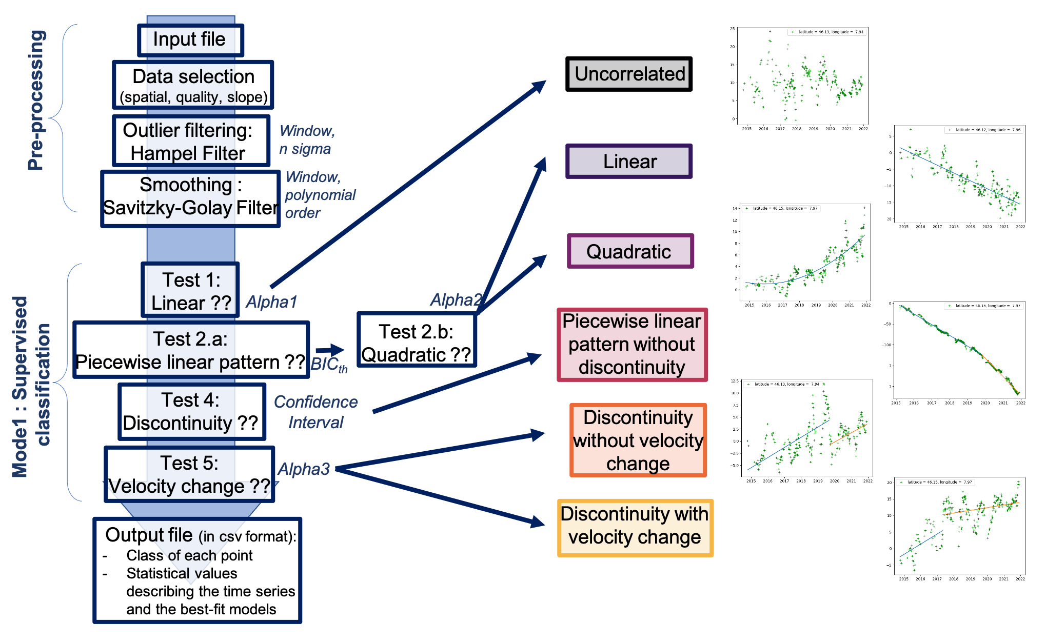
TimeSAT is a service developed by CNRS-EOST (Strasbourg, France) for classifying ground motion displacement time series in specific behaviors/patterns, detect changes in the time series (increase, decrease, periodicity) and identify spatial clusters of homogeneous styles of ground motion. The service currently allows ingesting PSInSAR and SBAS InSAR time series and optical offset-tracking time series. It consists of:

1. A module for data pre-processing (advanced Savitzky-Golay filtering, data subset masking);
2. A module for time series classification, for which several processing workflows are possible:

• Mode 1 / supervised: The classification in pre-defined distinctive patterns (uncorrelated trend, linear trend, quadratic trend, bilinear trend) based on a sequence of conditional statistical tests,
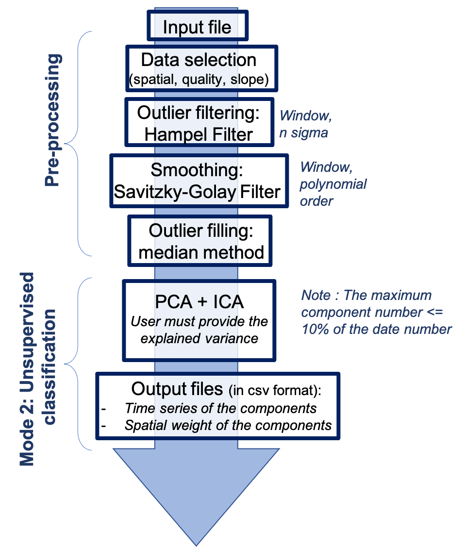
• Mode 2 / unsupervised: The classification using a combination of principal component analysis (IPA) and independent component analysis (ICA) to detect and classify specific patterns.

TimeSAT allows the processing of time series non structured and unevenly distributed in time and in space. The workflow is computationally optimized and parallelised and is implemented on the Mésocentre/HPC infrastructure of the University of Strasbourg. Thanks to the parallelization and scaling of the code, the processing of about 1 million time series (pixel, PS/DS points) of 5 a years period lasts less than 2 hours.

TimeSAT Pre-processing is using Python librairies based on [1] and [2],

TimeSAT Mode 1 implements part of the supervised classification approach described in [3] using advanced statistical tests [4], [5], [6],

TimeSAT Mode 2 implements unsupervised classification approaches such as those used by [7], [8] and [9].

EO sources supported:

• PSInSAR (Snapping FullRes, SqueeSAR, or any other PSInSAR methods) and SBAS InSAR time series. Format: standard Comma-Separated Values (.csv) format in geographic coordinates.
• Optical offset-tracking time series (GDM-OPT-SLIDE, GDM-OPT-ICE, or any other offset tracking methods). Format: standard Comma-Separated Values (.csv) format in geographic coordinates.

Output specifications

• Mode 1 / supervised classification: Format: standard Comma-Separated Values (.csv) format in geographic coordinates.
• Mode 2 / unsupervised classification: Format: standard Comma-Separated Values (CSV) format in geographic coordinates.
• One report (*.pdf file) summarizing the processing and presenting statistics on the results.

Processing workflows

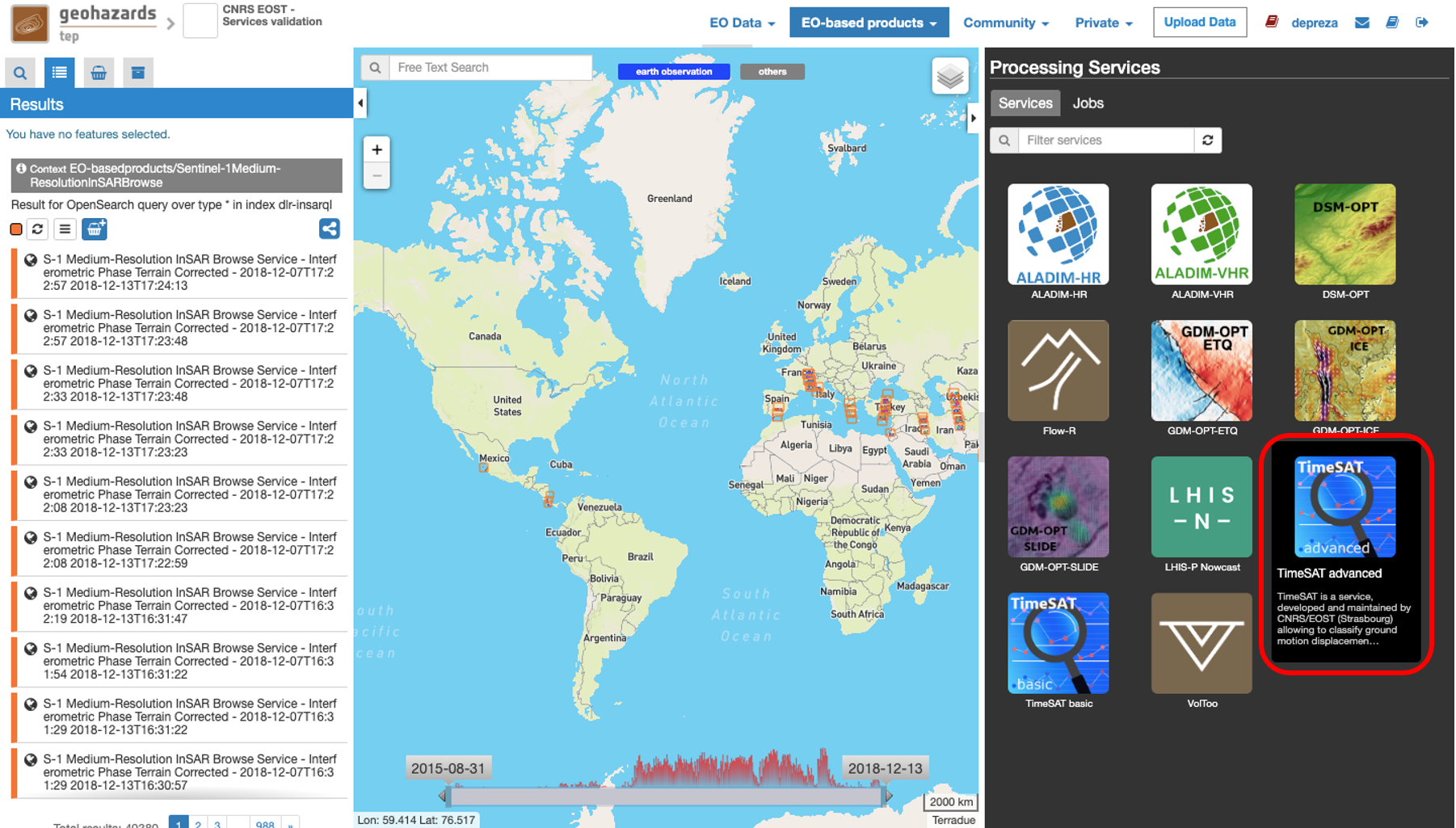
This tutorial introduces to the use of the ground motion classification service TimeSAT.

There are two versions available for the service (basic, advanced). This tutorial describes all the parameters and details the ones associated with the advanced version of the service.

Select the processing service¶

• Login to the platform (see user section)
• Go to the Geobrowser, expand the panel “Processing services” on the right hand side and select the processing service TimeSAT”:

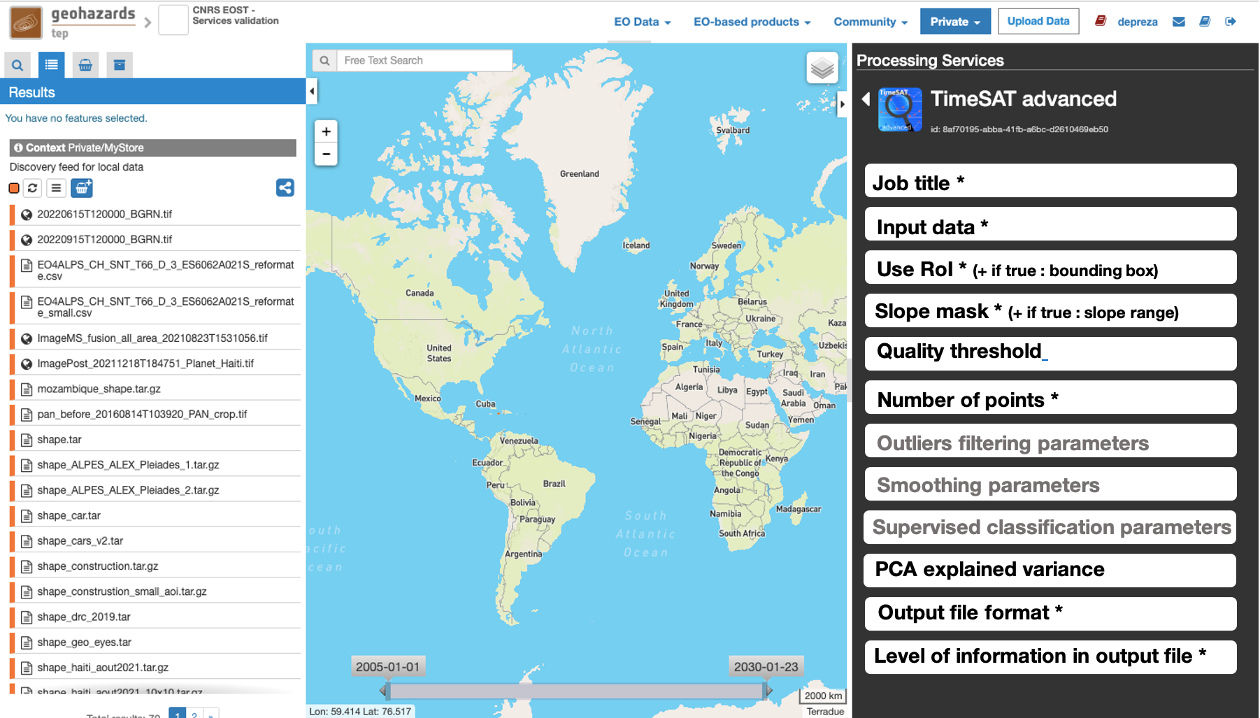
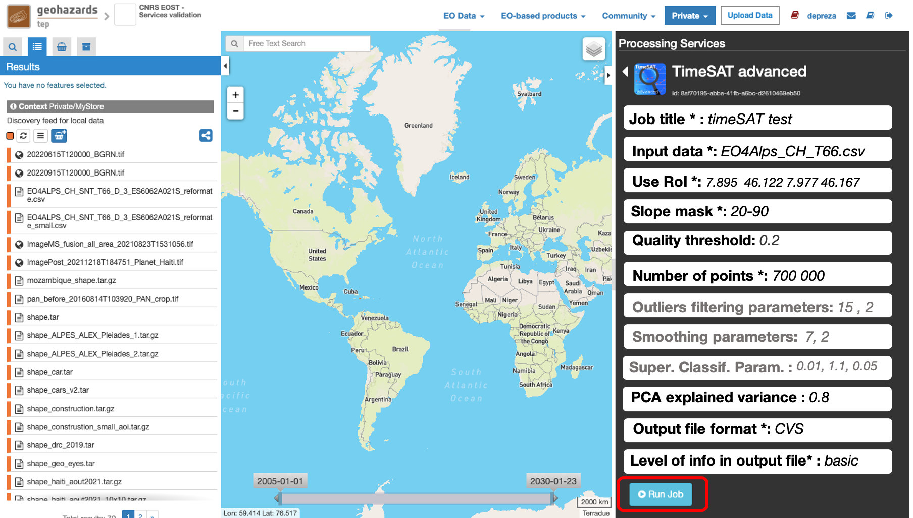
This will display the service panel including several (22 for the advanced mode, 13 for the basic mode) pre-defined parameters which can be adapted.

This figure displays all the parameters; the advanced parameters are indicated in grey color.

Select input data¶

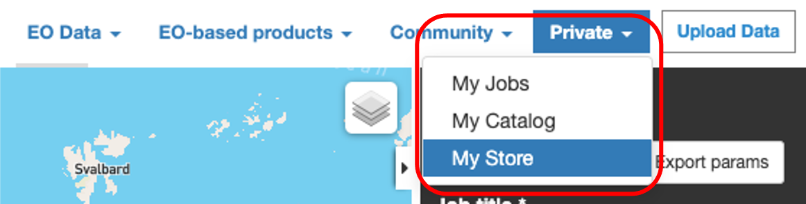
Select My store from the Private pulldown menu:

Drop the archive in the field of the service panel named “Input file”:

Set the processing parameters¶

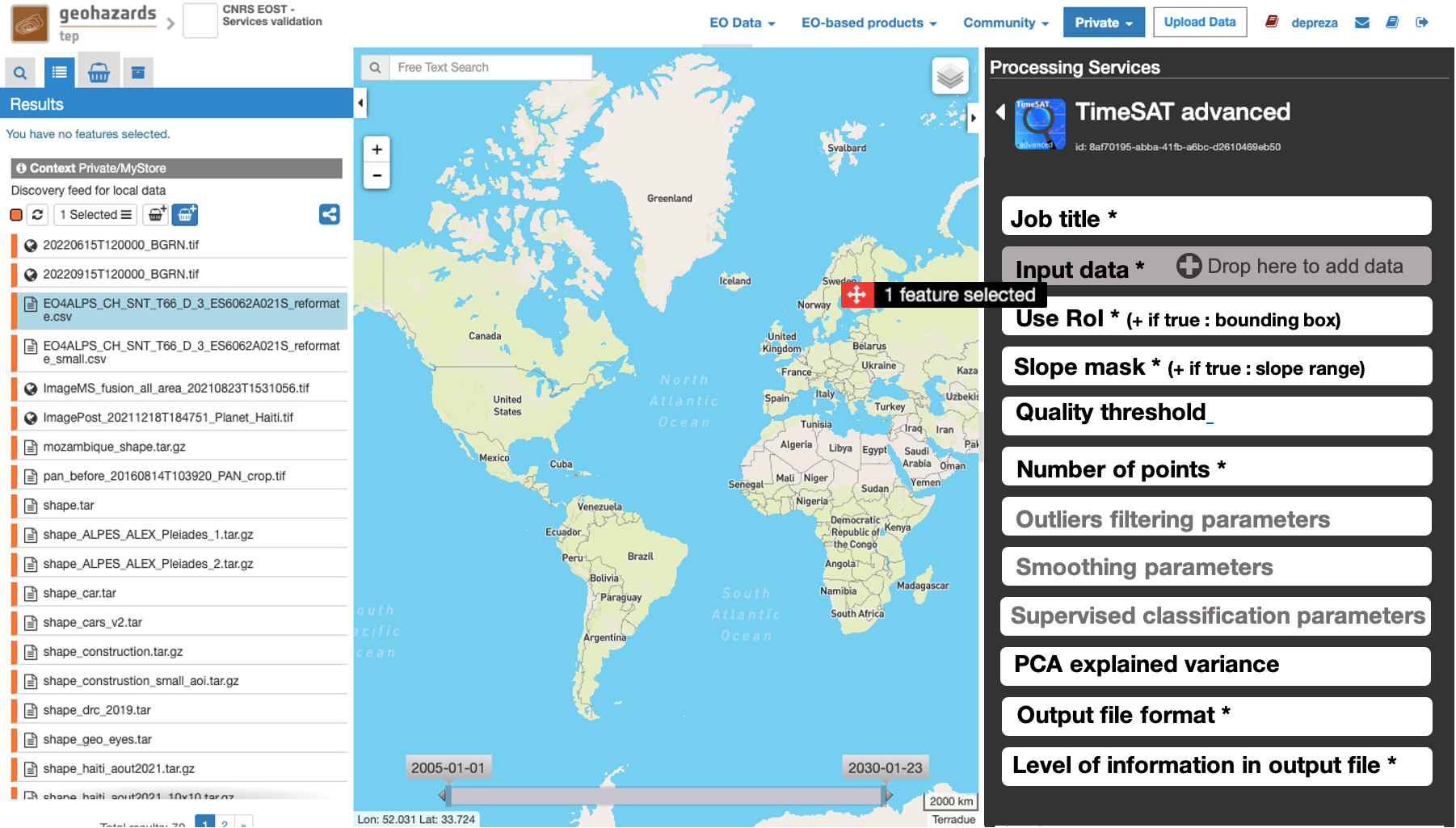
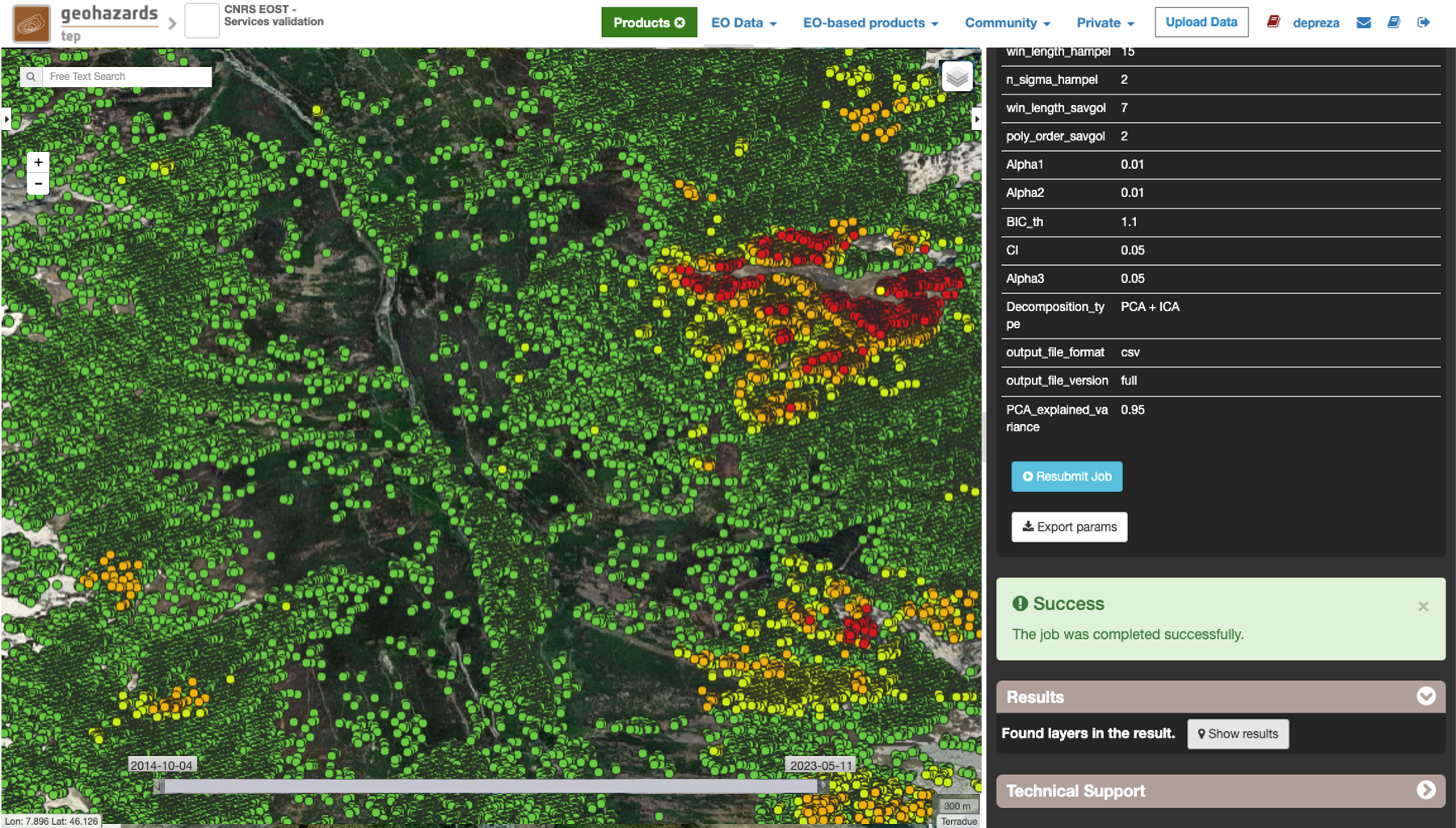
Some processing parameters can be adjusted. When hovering over the parameter fields, you will see a short explanation for each of the parameters.

General

• Job title: Defines the title of the job
• Input data: Input data in csv or kml format
• Time series classification approach: Type of classification approach (e.g. supervised / mode 1 or unsupervised /mode 2 pattern identification or both)

Data selection

• Use RoI (Region Of Interest) If set to True the spatial data selection is activated
• Region Of Interest bounding box Define the bounding box of the Region of Interest (RoI)
• Slope mask If set to True the data selection based on the slope in activated (Slope computed using Copernicus DEM)
• Slope mask: range minimum / maximum Defines the slope range for which the points are keeping
• Minimum quality threshold (coherence or correlation) Defines a minimum InSAR interferogram coherence OR coefficient of correlation for image correlation for which the points are keeping

Pre-processing

• Pre-processing: Length of filtering window for outlier removal Defines the length of the sliding window for outlier removal using Hampel identifier
• Pre-processing: Standard deviation value for outlier removal Defines the number of standard deviations to detect the outlier using Hampel identifier
• Pre-processing: Length of filtering window for time series smoothing Defines the length of filtering window (Savitzky-Golay filter): the value must be less than or equal to the number of dates in the time series
• Pre-processing: Polynomial order for time series smoothing Defines the order of the polynomial used for sample fitting (Savitzky-Golay filter): the value must be less than the length of the filtering window.

Mode 1: Supervised classification

• Supervised classification: Linear term level of significance Defines the linear ANOVA test threshold (α1): the time series is classified as uncorrelated pattern if α1 < p-value.
• Supervised classification: Quadratic term level of significance Defines the quadratic ANOVA test threshold (α2): the time series is classified as linear pattern if α2 < p-value.
• Supervised classification: Piecewise linear pattern level of significance Defines the BIC threshold (Bth): the time series is classified as piecewise linear pattern if the minimum BIC of segmented regression models is less than the BIC of quadratic and linear models and if the evidence ratio is > Bth.
• Supervised classification: Value for testing the significance of the discontinuity at the break point Defines the significance of vertical jump at the break point for segmented regression models
• Supervised classification: Value for testing the significance of velocity change Defines the linear ANOVA test threshold (α3): the velocity change is significant if there is a significant linear trend in the second part of the time series after linear modeling of the first part of the time series (α3 < p-value).

Mode 2: Unsupervised classification

• Unsupervised classification: PCA explained variance (used to determine the component number) Defines the desired percentage of explained variance by the usupervised analysis. It will allow to estimate the number of necessary components.

Non-expert users are advised to keep the default values or to use the basic version of the code.

Run the job¶

• You are good to go. Click on the button Run Job at the bottom of the right panel. Depending on the allocated resources the execution will require a few hours to terminate.

• Once the job has finished, click on the Show results button to get a list and a pre-visualization of the results.

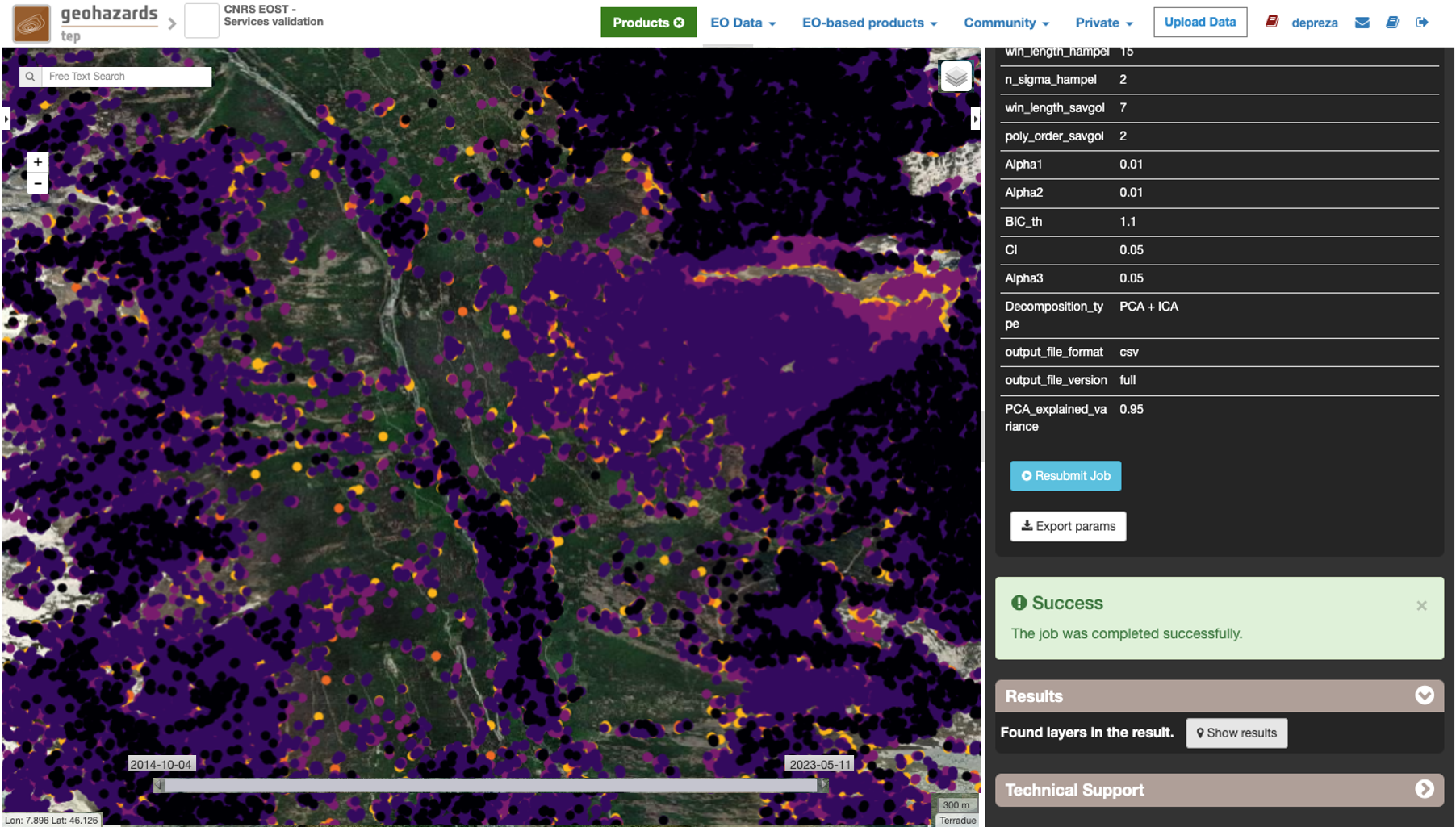
Note

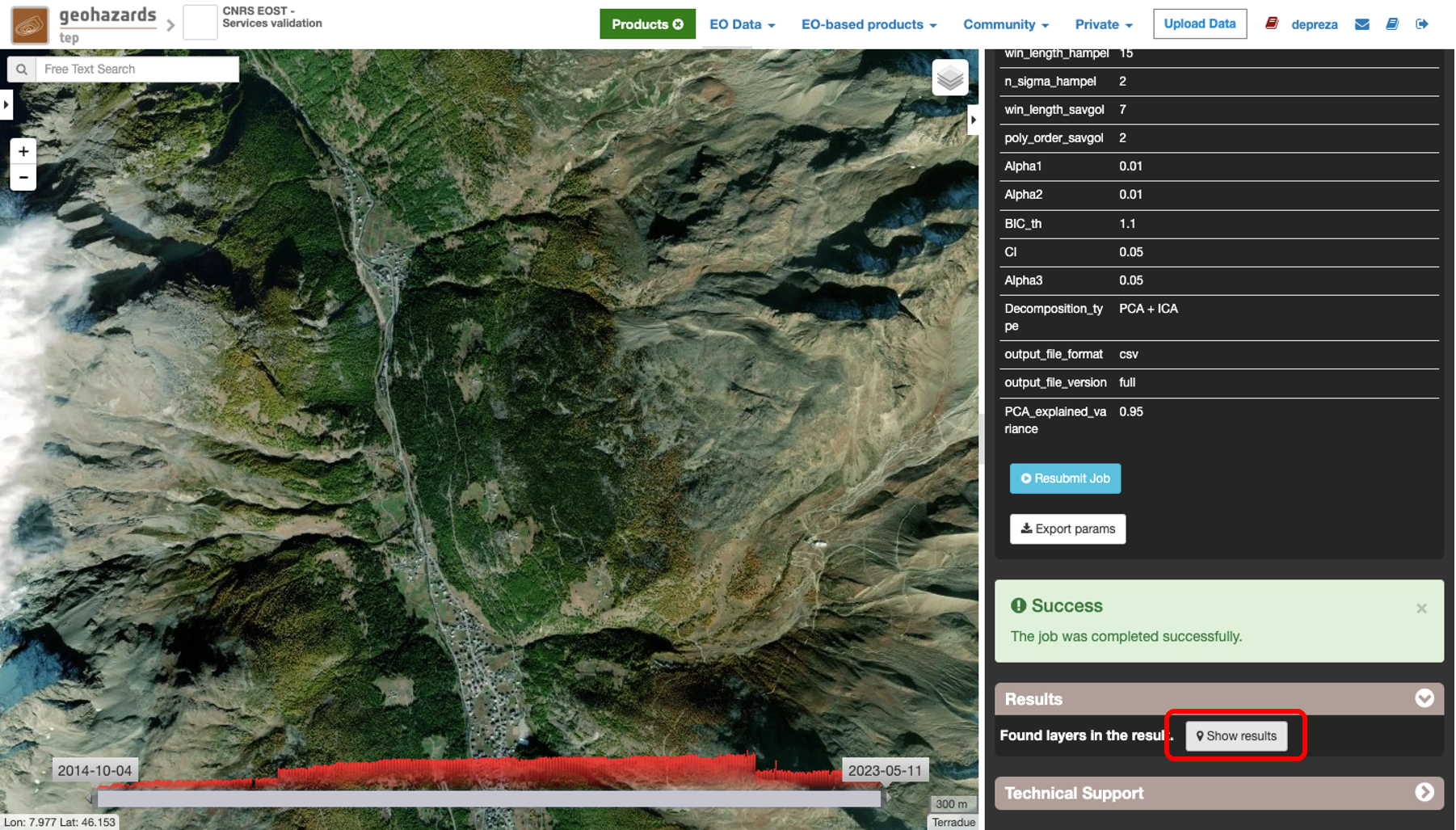
The pre-visualization in the Geobrowser is only a preview. To generate this preview the csv files are rasterized with a resolution of 0.0001°. For further analysis and post-processing, the results have to be donwloaded.

• Example of the classification obtained with Timesat / Mode 1 over the Jegihorn Landslide (Switzerland) with PSInSAR time series (SqueeSAR processing by TRE-Altamira.